非线性数据的多项式回归 - ML

日常生活中经常会遇到非线性数据。考虑物理学中研究的一些运动方程。

弹丸运动：弹丸的高度计算为 h = -½ gt ² +ut +ho
自由落体下的运动方程：物体在重力作用下自由落体't'秒后所经过的距离为 ½ gt ² 。
匀加速物体行进的距离：距离可以计算为 ut + ½at ²
在哪里，
g = acceleration due to gravity
u = initial velocity
ho = initial height
a = acceleration

编程需要懂一点英语

除了这些例子之外，在组织的生长速度、疾病流行的进展、黑体辐射、钟摆的运动等方面也观察到了非线性趋势。这些例子清楚地表明，我们之间不可能总是存在线性关系。独立属性和依赖属性。因此，线性回归对于处理这种非线性情况是一个糟糕的选择。这就是多项式回归来拯救我们的地方！！

多项式回归是一种强大的技术，可以解决存在二次、三次或更高阶非线性关系的情况。多项式回归的基本概念是将每个独立属性的幂添加为新属性，然后在此扩展的特征集合上训练线性模型。
让我们用一个例子来说明多项式回归的使用。考虑这样一种情况，其中因变量 y 相对于自变量 x 随关系变化

y = 13x2 + 2x + 7

我们将使用 Scikit-Learn 的PolynomialFeatures类来实现。

Step1：导入库并生成随机数据集。

# Importing the libraries
import numpy as np
import matplotlib.pyplot as plt
from sklearn.linear_model import LinearRegression
from sklearn.preprocessing import PolynomialFeatures
from sklearn.metrics import mean_squared_error, r2_score
  
# Importing the dataset
## x = data, y = quadratic equation
x = np.array(7 * np.random.rand(100, 1) - 3)
x1 = x.reshape(-1, 1)
y = 13 * x*x + 2 * x + 7

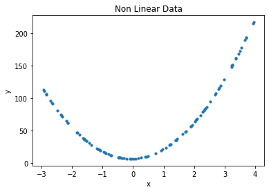
Step2：绘制数据点。

# data points
plt.scatter(x, y, s = 10)
plt.xlabel('x')
plt.ylabel('y')
plt.title('Non Linear Data')

Step3：首先尝试用线性模型拟合数据。

# Model initialization
regression_model = LinearRegression()
# Fit the data(train the model)
regression_model.fit(x1, y)
print('Slope of the line is', regression_model.coef_)
print('Intercept value is', regression_model.intercept_)
# Predict
y_predicted = regression_model.predict(x1)

输出：

Slope of the line is [[14.87780012]]
Intercept value is [58.31165769]

第 4 步：绘制数据点和线性线。

# data points
plt.scatter(x, y, s = 10)
plt.xlabel("$x$", fontsize = 18)
plt.ylabel("$y$", rotation = 0, fontsize = 18)
plt.title("data points")
  
# predicted values
plt.plot(x, y_predicted, color ='g')

输出：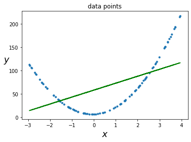

Equation of the linear model is y = 14.87x + 58.31

步骤 5：根据均方误差、均方根误差和 r2 分数计算模型的性能。

# model evaluation
mse = mean_squared_error(y, y_predicted)
  
rmse = np.sqrt(mean_squared_error(y, y_predicted))
r2 = r2_score(y, y_predicted)
  
# printing values
  
print('MSE of Linear model', mse)
  
print('R2 score of Linear model: ', r2)

输出：

MSE of Linear model 2144.8229656677095
R2 score of Linear model:  0.3019970606151057

线性模型的性能并不令人满意。让我们尝试 2 次多项式回归

第 6 步：为了提高性能，我们需要使模型稍微复杂一些。因此，让我们拟合一个 2 次多项式并进行线性回归。

poly_features = PolynomialFeatures(degree = 2, include_bias = False)
x_poly = poly_features.fit_transform(x1)
x[3]

输出：

Out[]:array([-2.84314447])

x_poly[3]

输出：

Out[]:array([-2.84314447,  8.08347046])

除了 x 列之外，还引入了另一列，即实际数据的平方。现在我们继续进行简单的线性回归

lin_reg = LinearRegression()
lin_reg.fit(x_poly, y)
print('Coefficients of x are', lin_reg.coef_)
print('Intercept is', lin_reg.intercept_)

输出：

Coefficients of x are [[ 2. 13.]]
Intercept is [7.]

这是所需的方程 13x ² + 2x + 7

第 7 步：绘制获得的二次方程。

x_new = np.linspace(-3, 4, 100).reshape(100, 1)
x_new_poly = poly_features.transform(x_new)
y_new = lin_reg.predict(x_new_poly)
plt.plot(x, y, "b.")
plt.plot(x_new, y_new, "r-", linewidth = 2, label ="Predictions")
plt.xlabel("$x_1$", fontsize = 18)
plt.ylabel("$y$", rotation = 0, fontsize = 18)
plt.legend(loc ="upper left", fontsize = 14)
  
plt.title("Quadratic_predictions_plot")
plt.show()

输出：

第八步：计算多项式回归得到的模型的性能。

y_deg2 = lin_reg.predict(x_poly)
# model evaluation
mse_deg2 = mean_squared_error(y, y_deg2)
  
r2_deg2 = r2_score(y, y_deg2)
  
# printing values
  
print('MSE of Polyregression model', mse_deg2)
  
print('R2 score of Linear model: ', r2_deg2)

输出：

MSE of Polyregression model 7.668437973562934e-28
R2 score of Linear model:  1.0

对于给定的二次方程，多项式回归模型的性能远优于线性回归模型。
重要事实：PolynomialFeatures (degree = d) 将包含 n 个特征的数组转换为包含(n + d) 的数组！ /d！嗯！特征。

结论：多项式回归是处理非线性数据的有效方法，因为它可以找到普通线性回归模型难以做到的特征之间的关系。