非线性回归示例 – ML

非线性回归是多项式回归的一种。它是一种对因变量和自变量之间的非线性关系进行建模的方法。当数据显示曲线趋势时使用它，与非线性回归相比，线性回归不会产生非常准确的结果。这是因为在线性回归中，预先假设数据是线性的。

代码：

Python3

import numpy as np
import pandas as pd
 
# downloading dataset
! wget -nv -O china_gdp.csv https://s3-api.us-geo.objectstorage.softlayer.net/
                    cf-courses-data/CognitiveClass/ML0101ENv3/labs/china_gdp.csv
     
df = pd.read_csv("china_gdp.csv")
 
def sigmoid(x, Beta_1, Beta_2):
     y = 1 / (1 + np.exp(-Beta_1*(x-Beta_2)))
     return y
     
beta_1 = 0.10
beta_2 = 1990.0
 
# logistic function
Y_pred = sigmoid(x_data, beta_1, beta_2)
 
# plot initial prediction against datapoints
plt.plot(x_data, Y_pred * 15000000000000.)
plt.plot(x_data, y_data, 'ro')

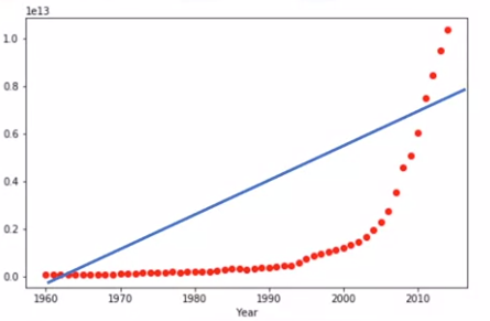
散点图显示了一个国家的 GDP 和时间之间的关系，但这种关系不是线性的。相反，在 2005 年之后，这条线开始变成曲线，不再遵循直线直线路径。在这种情况下，需要一种称为非线性回归的特殊估计方法。

代码：

Python3

import numpy as np
import pandas as pd
 
# downloading dataset
! wget -nv -O china_gdp.csv https://s3-api.us-geo.objectstorage.softlayer.net/
         cf-courses-data / CognitiveClass / ML0101ENv3 / labs / china_gdp.csv
     
df = pd.read_csv("china_gdp.csv")
 
def sigmoid(x, Beta_1, Beta_2):
     y = 1 / (1 + np.exp(-Beta_1*(x-Beta_2)))
     return y
      
x = np.linspace(1960, 2015, 55)
x = x / max(x)
y = sigmoid(x, *popt)
 
plt.figure(figsize =(8, 5))
plt.plot(xdata, ydata, 'ro', label ='data')
plt.plot(x, y, linewidth = 3.0, label ='fit')
plt.legend(loc ='best')
plt.ylabel('GDP')
plt.xlabel('Year')
plt.show()

输出：

存在许多不同的回归，可用于根据我们的要求无限度地拟合数据集的任何外观，例如二次回归、三次回归等。

代码：

Python3

import numpy as np
import matplotlib.pyplot as plt % matplotlib inline
 
x = np.arange(-5.0, 5.0, 0.1)
 
## You can adjust the slope and intercept to verify the changes in the graph
y = 2*(x) + 3
y_noise = 2 * np.random.normal(size = x.size)
ydata = y + y_noise
# plt.figure(figsize =(8, 6))
plt.plot(x, ydata,  'bo')
plt.plot(x, y, 'r')
plt.ylabel('Dependent Variable')
plt.xlabel('Independent Variable')
plt.show()

输出：

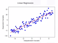
线性回归

代码：

Python3

import numpy as np
import matplotlib.pyplot as plt % matplotlib inline
 
x = np.arange(-5.0, 5.0, 0.1)
 
## You can adjust the slope and intercept to verify the changes in the graph
 
y = np.power(x, 2)
y_noise = 2 * np.random.normal(size = x.size)
ydata = y + y_noise
plt.plot(x, ydata,  'bo')
plt.plot(x, y, 'r')
plt.ylabel('Dependent Variable')
plt.xlabel('Independent Variable')
plt.show()

输出：

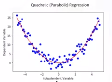
二次回归

代码：

Python3

import numpy as np
import matplotlib.pyplot as plt % matplotlib inline
 
x = np.arange(-5.0, 5.0, 0.1)
 
## You can adjust the slope and intercept to verify the changes in the graph
y = 1*(x**3) + 1*(x**2) + 1 * x + 3
y_noise = 20 * np.random.normal(size = x.size)
ydata = y + y_noise
plt.plot(x, ydata,  'bo')
plt.plot(x, y, 'r')
plt.ylabel('Dependent Variable')
plt.xlabel('Independent Variable')
plt.show()

输出：

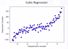
三次回归

我们可以称所有这些多项式回归，其中自变量 X 和因变量 Y 之间的关系被建模为 X 中的 N 次多项式。

多项式回归

对于被认为是非线性的模型，Y hat 必须是参数 Theta 的非线性函数，不一定是特征 X。当涉及到非线性方程时，它可以是指数、对数和物流，或许多其他类型。

输出：

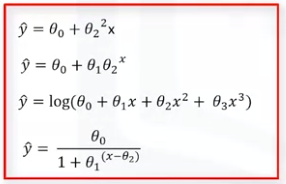
非线性回归方程

正如您在所有这些方程中看到的那样，Y 帽子的变化取决于参数 Theta 的变化，不一定只取决于 X。也就是说，在非线性回归中，模型在参数上是非线性的。