R 编程中的多项式回归

多项式回归是线性回归的一种形式，其中自变量 x 和因变量 y 之间的关系被建模为 n 次多项式。多项式回归拟合 x 的值与 y 的相应条件均值之间的非线性关系，表示为 E(y|x)。基本上，它将二次或多项式项添加到回归中。通常，这种回归用于一个结果变量和一个预测变量。

多项式回归的需要

• 与线性数据集不同，如果试图将线性模型应用到非线性数据集上而不做任何修改，那么将会产生非常不令人满意和剧烈的结果。
• 这可能会导致损失函数增加、准确率下降和错误率高。
• 与线性模型不同，多项式模型涵盖了更多的数据点。

多项式回归的应用

通常，多项式回归用于以下场景：

• 组织的生长速度。
• 与疾病有关的流行病的进展。
• 湖泊沉积物中碳同位素分布现象[J].

R编程中多项式回归的解释

多项式回归也称为多项式线性回归，因为它取决于线性排列的系数而不是变量。在 R 中，如果想要实现多项式回归，那么他必须安装以下软件包：

• tidyverse包，用于更好的可视化和操作。
• 插入符号包，可实现更流畅、更轻松的机器学习工作流程。

正确安装软件包后，需要正确设置数据。为此，第一个需要将数据分成两组（训练集和测试集）。然后可以将数据可视化为各种图表。在 R 中，为了拟合多项式回归，第一个需要使用set.seed(n)函数生成伪随机数。

多项式回归将多项式或二次项添加到回归方程中，如下所示：

medv = b0 + b1 * lstat + b2 * lstat ²

where

mdev: is the median house value

lstat: is the predictor variable

在 R 中，要创建预测变量 x ² ，应使用函数I() ，如下所示： I(x ² ) 。这将 x 提高到 2 次方。多项式回归可以在 R 中计算如下：

lm(medv ~ lstat + I(lstat^2), data = train.data)

对于以下示例，让我们以 MASS 包的波士顿数据集为例。

例子：

r

# R program to illustrate
# Polynomial regression
 
# Importing required library
library(tidyverse)
library(caret)
theme_set(theme_classic())
 
# Load the data
data("Boston", package = "MASS")
# Split the data into training and test set
set.seed(123)
training.samples <- Boston$medv %>%
  createDataPartition(p = 0.8, list = FALSE)
train.data  <- Boston[training.samples, ]
test.data <- Boston[-training.samples, ]
 
# Build the model
model <- lm(medv ~ poly(lstat, 5, raw = TRUE),
            data = train.data)
# Make predictions
predictions <- model %>% predict(test.data)
# Model performance
modelPerfomance = data.frame(
                    RMSE = RMSE(predictions, test.data$medv),
                     R2 = R2(predictions, test.data$medv)
                 )
 
print(lm(medv ~ lstat + I(lstat^2), data = train.data))
print(modelPerfomance)

输出：

Call:
lm(formula = medv ~ lstat + I(lstat^2), data = train.data)

Coefficients:
(Intercept)        lstat     I(lstat^2)  
    42.5736       -2.2673       0.0412  

      RMSE        R2
1   5.270374 0.6829474

多项式回归的图形绘制

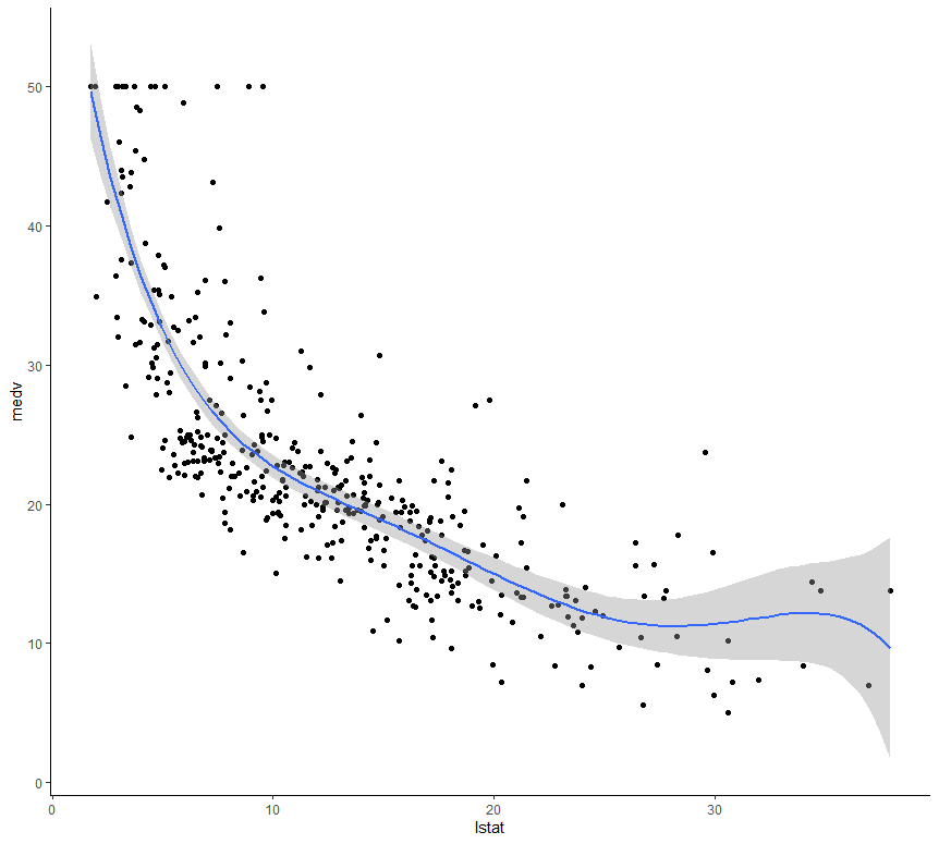
在 R 中，如果想为实现多项式回归时生成的输出绘制图表，他可以使用ggplot()函数。

例子：

r

# R program to illustrate
# Graph plotting in
# Polynomial regression
 
# Importing required library
library(tidyverse)
library(caret)
theme_set(theme_classic())
 
# Load the data
data("Boston", package = "MASS")
# Split the data into training and test set
set.seed(123)
training.samples <- Boston$medv %>%
  createDataPartition(p = 0.8, list = FALSE)
train.data  <- Boston[training.samples, ]
test.data <- Boston[-training.samples, ]
 
# Build the model
model <- lm(medv ~ poly(lstat, 5, raw = TRUE), data = train.data)
# Make predictions
predictions <- model %>% predict(test.data)
# Model performance
data.frame(RMSE = RMSE(predictions, test.data$medv),
           R2 = R2(predictions, test.data$medv))
   
ggplot(train.data, aes(lstat, medv) ) + geom_point() +
stat_smooth(method = lm, formula = y ~ poly(x, 5, raw = TRUE))

输出：