ML | Python的小批量梯度下降

📌 相关文章

📜 ML | Python的小批量梯度下降

📅 最后修改于: 2021-04-17 02:45:06 🧑 作者: Mango

在机器学习中，梯度下降是一种用于计算模型参数(系数和偏差)的优化技术，用于线性回归，对数回归，神经网络等算法。在此技术中，我们反复遍历训练集并更新模型相对于训练集的误差梯度的参数。

根据更新模型参数时考虑的训练示例数量，我们有3种类型的梯度下降：

批次梯度下降：在计算相对于整个训练集的误差梯度之后，更新参数
随机梯度下降：在针对单个训练示例计算误差梯度之后更新参数
迷你批量梯度下降：在计算相对于训练集的子集的误差梯度之后，更新参数

Batch Gradient Descent	Stochastic Gradient Descent	Mini-Batch Gradient Descent
Since entire training data is considered before taking a step in the direction of gradient, therefore it takes a lot of time for making a single update.	Since only a single training example is considered before taking a step in the direction of gradient, we are forced to loop over the training set and thus cannot exploit the speed associated with vectorizing the code.	Since a subset of training examples is considered, it can make quick updates in the model parameters and can also exploit the speed associated with vectorizing the code.
It makes smooth updates in the model parameters	It makes very noisy updates in the parameters	Depending upon the batch size, the updates can be made less noisy – greater the batch size less noisy is the update

因此，小批量梯度下降在快速收敛和与梯度更新相关的噪声之间做出了折衷，这使其成为一种更加灵活和健壮的算法。

小批量梯度下降：

算法-

Let theta = model parameters and max_iters = number of epochs.

for itr = 1, 2, 3, …, max_iters:
for mini_batch (X_mini, y_mini):

Forward Pass on the batch X_mini:
- Make predictions on the mini-batch
- Compute error in predictions (J(theta)) with the current values of the parameters
Backward Pass:
- Compute gradient(theta) = partial derivative of J(theta) w.r.t. theta
Update parameters:
- theta = theta – learning_rate*gradient(theta)

为什么编程需要懂一点英语

以下是Python实现：

步骤＃1：第一步是导入依赖关系，生成用于线性回归的数据并可视化生成的数据。我们已经生成了8000个数据示例，每个示例都有2个属性/功能。这些数据示例进一步分为分别具有7200和800个示例的训练集(X_train，y_train)和测试集(X_test，y_test)。

# importing dependencies
import numpy as np
import matplotlib.pyplot as plt
  
# creating data
mean = np.array([5.0, 6.0])
cov = np.array([[1.0, 0.95], [0.95, 1.2]])
data = np.random.multivariate_normal(mean, cov, 8000)
  
# visualising data
plt.scatter(data[:500, 0], data[:500, 1], marker = '.')
plt.show()
  
# train-test-split
data = np.hstack((np.ones((data.shape[0], 1)), data))
  
split_factor = 0.90
split = int(split_factor * data.shape[0])
  
X_train = data[:split, :-1]
y_train = data[:split, -1].reshape((-1, 1))
X_test = data[split:, :-1]
y_test = data[split:, -1].reshape((-1, 1))
  
print("Number of examples in training set = % d"%(X_train.shape[0]))
print("Number of examples in testing set = % d"%(X_test.shape[0]))

输出：

训练集中的示例数= 7200
测试集中的示例数= 800

步骤＃2：接下来，我们编写代码以使用小批量梯度下降实现线性回归。
gradientDescent()是主要驱动函数和其它功能是用于进行预测的辅助功能- hypothesis() ，计算梯度- gradient()计算误差- cost()和创建微型批次- create_mini_batches()驱动程序函数将初始化参数，为模型计算最佳的参数集，然后将这些参数以及包含错误历史记录的列表返回，这些列表将随着参数的更新而更新。

# linear regression using "mini-batch" gradient descent
# function to compute hypothesis / predictions
def hypothesis(X, theta):
    return np.dot(X, theta)
  
# function to compute gradient of error function w.r.t. theta
def gradient(X, y, theta):
    h = hypothesis(X, theta)
    grad = np.dot(X.transpose(), (h - y))
    return grad
  
# function to compute the error for current values of theta
def cost(X, y, theta):
    h = hypothesis(X, theta)
    J = np.dot((h - y).transpose(), (h - y))
    J /= 2
    return J[0]
  
# function to create a list containing mini-batches
def create_mini_batches(X, y, batch_size):
    mini_batches = []
    data = np.hstack((X, y))
    np.random.shuffle(data)
    n_minibatches = data.shape[0] // batch_size
    i = 0
  
    for i in range(n_minibatches + 1):
        mini_batch = data[i * batch_size:(i + 1)*batch_size, :]
        X_mini = mini_batch[:, :-1]
        Y_mini = mini_batch[:, -1].reshape((-1, 1))
        mini_batches.append((X_mini, Y_mini))
    if data.shape[0] % batch_size != 0:
        mini_batch = data[i * batch_size:data.shape[0]]
        X_mini = mini_batch[:, :-1]
        Y_mini = mini_batch[:, -1].reshape((-1, 1))
        mini_batches.append((X_mini, Y_mini))
    return mini_batches
  
# function to perform mini-batch gradient descent
def gradientDescent(X, y, learning_rate = 0.001, batch_size = 32):
    theta = np.zeros((X.shape[1], 1))
    error_list = []
    max_iters = 3
    for itr in range(max_iters):
        mini_batches = create_mini_batches(X, y, batch_size)
        for mini_batch in mini_batches:
            X_mini, y_mini = mini_batch
            theta = theta - learning_rate * gradient(X_mini, y_mini, theta)
            error_list.append(cost(X_mini, y_mini, theta))
  
    return theta, error_list

调用gradientDescent()函数以计算模型参数(θ)并可视化误差函数的变化。

theta, error_list = gradientDescent(X_train, y_train)
print("Bias = ", theta[0])
print("Coefficients = ", theta[1:])
  
# visualising gradient descent
plt.plot(error_list)
plt.xlabel("Number of iterations")
plt.ylabel("Cost")
plt.show()

输出：
偏差= [0.81830471]
系数= [[1.04586595]]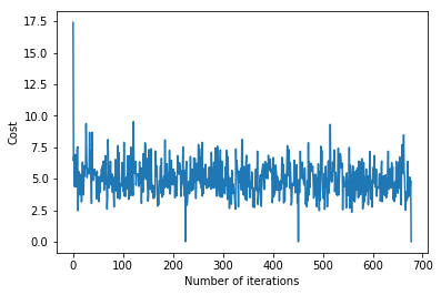

步骤＃3：最后，我们对测试集进行预测并计算预测中的平均绝对误差。

# predicting output for X_test
y_pred = hypothesis(X_test, theta)
plt.scatter(X_test[:, 1], y_test[:, ], marker = '.')
plt.plot(X_test[:, 1], y_pred, color = 'orange')
plt.show()
  
# calculating error in predictions
error = np.sum(np.abs(y_test - y_pred) / y_test.shape[0])
print("Mean absolute error = ", error)

输出：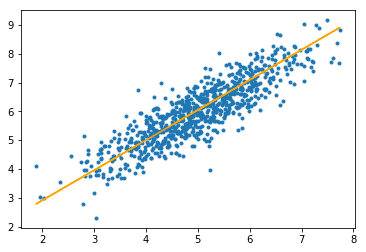

平均绝对误差= 0.4366644295854125

橙色线代表最终的假设函数： theta [0] + theta [1] * X_test [:, 1] + theta [2] * X_test [:, 2] = 0