梯度下降的矢量化

在机器学习中，回归问题可以通过以下方式解决：

1. 使用优化算法——梯度下降

• 批量梯度下降。
• 随机梯度下降。
• 小批量梯度下降
• 其他高级优化算法，如（共轭下降……）

2. 使用正态方程：

• 使用线性代数的概念。

让我们考虑单变量线性回归问题的批量梯度下降的情况。

这个回归问题的成本函数是：

$J(\Theta)=(1/2m)*\sum_{i=1}^m(h_{\theta}(x^i)-y^i)^2$

目标：

$minimize_{\ \theta_{o},\theta_{1}}\ \ J({\theta})$

为了解决这个问题，我们可以采用矢量化方法（使用线性代数的概念）或非矢量化方法（使用 for 循环）。

1. 非向量化方法：

这里为了解决下面提到的数学表达式，我们使用for 循环。

The above mathematical expression is a part of Cost Function.

$\sum_{i=1}^m(h_{\theta}(x^i)-y^i)^2$

The above Mathematical Expression is the hypothesis.

$h_{\theta}=\theta_{0}x_{0}+\theta_{1}x_{1}+\theta_{2}x_{2}+... +\theta_{n}x_{n}\\ where,\\ h_{\theta}=hypothesis.\\$

代码：Unvectorzed Grad 的Python实现

# Import required modules.
from sklearn.datasets import make_regression
import matplotlib.pyplot as plt
import numpy as np
import time
   
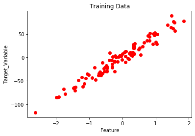
# Create and plot the data set.
x, y = make_regression(n_samples = 100, n_features = 1,
                       n_informative = 1, noise = 10, random_state = 42)
  
plt.scatter(x, y, c = 'red')
plt.xlabel('Feature')
plt.ylabel('Target_Variable')
plt.title('Training Data')
plt.show()
  
# Convert y from 1d to 2d array.
y = y.reshape(100, 1)
   
# Number of Iterations for Gradient Descent
num_iter = 1000
   
# Learning Rate
alpha = 0.01
   
# Number of Training samples.
m = len(x)
   
# Initializing Theta.
theta = np.zeros((2, 1),dtype = float)
   
# Variables
t0 = t1 = 0
Grad0 = Grad1 = 0
  
# Batch Gradient Descent.
start_time = time.time()
   
for i in range(num_iter):
    # To find Gradient 0.
    for j in range(m):
        Grad0 = Grad0 + (theta[0] + theta[1] * x[j]) - (y[j])
      
    # To find Gradient 1.
    for k in range(m):
        Grad1 = Grad1 + ((theta[0] + theta[1] * x[k]) - (y[k])) * x[k]
    t0 = theta[0] - (alpha * (1/m) * Grad0)
    t1 = theta[1] - (alpha * (1/m) * Grad1)
    theta[0] = t0
    theta[1] = t1
    Grad0 = Grad1 = 0
       
# Print the model parameters.    
print('model parameters:',theta,sep = '\n')
   
# Print Time Take for Gradient Descent to Run.
print('Time Taken For Gradient Descent in Sec:',time.time()- start_time)
  
# Prediction on the same training set.
h = []
for i in range(m):
    h.append(theta[0] + theta[1] * x[i])
       
# Plot the output.
plt.plot(x,h)
plt.scatter(x,y,c = 'red')
plt.xlabel('Feature')
plt.ylabel('Target_Variable')
plt.title('Output')

输出：

model parameters:
[[ 1.15857049]
 [44.42210912]]
 
Time Taken For Gradient Descent in Sec: 2.482538938522339

2.矢量化方法：

这里为了解决下面提到的数学表达式，我们使用矩阵和向量（线性代数）。

The above mathematical expression is a part of Cost Function.

$\sum_{i=1}^m(h_{\theta}(x^i)-y^i)^2$

The above Mathematical Expression is the hypothesis.

$h_{\theta}=\theta^T.X\\ where,\\ h_{\theta}=hypothesis.\\ \theta= \begin{bmatrix} \theta_{0} \\ \theta_{1}\\ \theta_{2}\\ \theta_{3}\\ .\\ .\\ \theta_{n}\\ \end{bmatrix} X= \begin{bmatrix} {x_{0}} \\ {x_{1}}\\ {x_{2}}\\ {x_{3}}\\ .\\ .\\ {x_{n}}\\ \end{bmatrix}\\$

批量梯度下降：

$Loop\ until\ converge\{\\ \ \theta_{j}:=\theta_{j}-(1/m)*(\alpha)*\frac{\partial J(\theta)}{\partial \theta_{j}} \\ \}\\ Let, \ Gradients=\frac{\partial J(\theta)}{\partial \theta_{j}}$

使用矩阵运算查找梯度的概念：

$X\_New= \begin{bmatrix} {x_{0}^1} & {x_{1}^1} \\ {x_{0}^2} & {x_{1}^2}\\ {x_{0}^3} & {x_{1}^3}\\ {x_{0}^4} & {x_{1}^4}\\ . & .\\ . & .\\ . & .\\ {x_{0}^m} & {x_{1}^m} \end{bmatrix}_{m X 2} \theta= \begin{bmatrix} \theta_{0} \\ \theta_{1}\\ \end{bmatrix}_{2X1}\\ where,\\ \x_{0}^i=1\\$

$H(\theta)=X\_New\ .\ \theta\\ H(\theta)= \begin{bmatrix} {\Theta_{0}}{x_{0}^1}+{\Theta_{1}}{x_{1}^1} \\ {\Theta_{0}}{x_{0}^2}+{\Theta_{1}}{x_{1}^2}\\ {\Theta_{0}}{x_{0}^3}+{\Theta_{1}}{x_{1}^3}\\ {\Theta_{0}}{x_{0}^4}+{\Theta_{1}}{x_{1}^4}\\ .\\ .\\ . \\ {\Theta_{0}}{x_{0}^m}+{\Theta_{1}}{x_{1}^m} \end{bmatrix}_{mX1} And\ \ \ Y= \begin{bmatrix} {y^1}\\ {y^2}\\ {y^3}\\ .\\ .\\ .\\ {y^m} \end{bmatrix}_{mX1}\\$

$H(\theta)-Y= \begin{bmatrix} {\Theta_{0}}{x_{0}^1}+{\Theta_{1}}{x_{1}^1} -y^1\\ {\Theta_{0}}{x_{0}^2}+{\Theta_{1}}{x_{1}^2}-y^2\\ {\Theta_{0}}{x_{0}^3}+{\Theta_{1}}{x_{1}^3}-y^3\\ {\Theta_{0}}{x_{0}^4}+{\Theta_{1}}{x_{1}^4}-y^4\\ .\\ .\\ . \\ {\Theta_{0}}{x_{0}^m}+{\Theta_{1}}{x_{1}^m}-y^m \end{bmatrix}_{mX1} \\$

$X\_New^T= \begin{bmatrix} {x_{0}^1\ x_{0}^2\ x_{0}^3\ .\ .\ .\ x_{0}^m}\\ {x_{1}^1\ x_{1}^2\ x_{1}^3\ .\ .\ .\ x_{1}^m} \end{bmatrix}_{2Xm} \\$

$Gradients=X\_New\ . \ (H(\theta)-Y)\\ = \begin{bmatrix} {x_{0}^1(\Theta x_{0}^1+\Theta x_{1}^1-y^1)\ + \ x_{0}^2(\Theta x_{0}^2+\Theta x_{1}^2-y^2)\ + \ x_{0}^3(\Theta x_{0}^3+\Theta x_{1}^3-y^3)\ + . . .}\\ {x_{1}^1(\Theta x_{0}^1+\Theta x_{1}^1-y^1)\ + \ x_{1}^2(\Theta x_{0}^2+\Theta x_{1}^2-y^2)\ + \ x_{1}^3(\Theta x_{0}^3+\Theta x_{1}^3-y^3)\ + . . .}\\ \end{bmatrix}_{2X1}\\$

$Finally\ we\ can \ say,\\ \ \ \ Gradients=\frac{\partial J(\theta)}{\partial \theta_{j}}=X\_New^T.(X\_New.\theta-Y)$

代码：矢量化梯度下降方法的Python实现

# Import required modules.
from sklearn.datasets import make_regression
import matplotlib.pyplot as plt
import numpy as np
import time
   
# Create and plot the data set.
x, y = make_regression(n_samples = 100, n_features = 1,
                       n_informative = 1, noise = 10, random_state = 42)
  
plt.scatter(x, y, c = 'red')
plt.xlabel('Feature')
plt.ylabel('Target_Variable')
plt.title('Training Data')
plt.show()
  
  
# Adding x0=1 column to x array.
X_New = np.array([np.ones(len(x)), x.flatten()]).T
  
# Convert y from 1d to 2d array.
y = y.reshape(100, 1)
   
# Number of Iterations for Gradient Descent
num_iter = 1000
   
# Learning Rate
alpha = 0.01
   
# Number of Training samples.
m = len(x)
   
# Initializing Theta.
theta = np.zeros((2, 1),dtype = float)
   
# Batch-Gradient Descent.
start_time = time.time()
   
for i in range(num_iter):
    gradients = X_New.T.dot(X_New.dot(theta)- y)
    theta = theta - (1/m) * alpha * gradients
   
# Print the model parameters.    
print('model parameters:',theta,sep = '\n')
   
# Print Time Take for Gradient Descent to Run.
print('Time Taken For Gradient Descent in Sec:',time.time() - start_time)
  
# Hypothesis.
h = X_New.dot(theta) # Prediction on training data itself.
   
# Plot the Output.
plt.scatter(x, y, c = 'red')
plt.plot(x ,h)
plt.xlabel('Feature')
plt.ylabel('Target_Variable')
plt.title('Output')

输出：

model parameters:
[[ 1.15857049]
 [44.42210912]]
 
Time Taken For Gradient Descent in Sec: 0.019551515579223633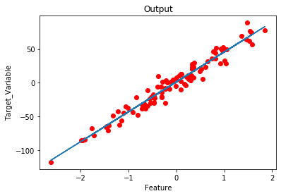

观察：

1. 实施矢量化方法减少了执行梯度下降（高效代码）所需的时间。
2. 易于调试。