线性回归中的梯度下降
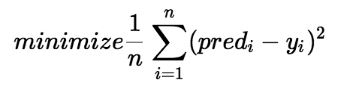
在线性回归中,模型的目标是根据给定的输入值 (x) 获得最佳拟合回归线来预测 y 的值。在训练模型时,模型会计算成本函数,该函数测量预测值 (pred) 和真实值 (y) 之间的均方根误差。该模型的目标是最小化成本函数。
为了最小化成本函数,模型需要具有最佳值 θ 1和 θ 2 。最初模型随机选择 θ 1和 θ 2值,然后迭代更新这些值以最小化成本函数,直到达到最小值。当模型达到最小成本函数时,它将具有最佳的 θ 1和 θ 2值。在线性方程的假设方程中使用这些最终更新的 θ 1和 θ 2值,模型以最佳方式预测 x 的值。
因此,问题出现了——如何更新 θ 1和 θ 2值?
线性回归成本函数:

线性回归的梯度下降算法
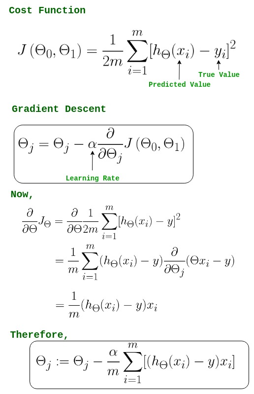
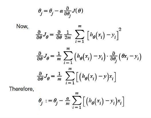
-> θj     : Weights of the hypothesis.
-> hθ(xi) : predicted y value for ith input.
-> j     : Feature index number (can be 0, 1, 2, ......, n).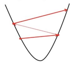
-> α : Learning Rate of Gradient Descent.我们将成本函数绘制为参数估计的函数,即假设函数的参数范围和选择一组特定参数所产生的成本。我们向下移动到图中的坑,以找到最小值。这样做的方法是采用成本函数的导数,如上图所示。梯度下降沿最陡下降的方向逐步降低成本函数。每个步骤的大小由称为学习率的参数α决定。
在梯度下降算法中,可以推断出两点:
- 如果斜率为 +ve : θ j = θ j –(+ve 值)。因此θ j的值减小。
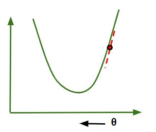
- 如果斜率为 -ve : θ j = θ j –(-ve 值)。因此θ j的值增加。

选择正确的学习率非常重要,因为它可以确保梯度下降在合理的时间内收敛。 :
- 如果我们选择α 很大,梯度下降会超过最小值。它可能无法收敛甚至发散。
- 如果我们选择 α 非常小,梯度下降将采取小步长达到局部最小值,并且需要更长的时间才能达到最小值。

对于线性回归成本,函数图始终是凸形的。
Python3
# Implementation of gradient descent in linear regression
import numpy as np
import matplotlib.pyplot as plt
class Linear_Regression:
def __init__(self, X, Y):
self.X = X
self.Y = Y
self.b = [0, 0]
def update_coeffs(self, learning_rate):
Y_pred = self.predict()
Y = self.Y
m = len(Y)
self.b[0] = self.b[0] - (learning_rate * ((1/m) *
np.sum(Y_pred - Y)))
self.b[1] = self.b[1] - (learning_rate * ((1/m) *
np.sum((Y_pred - Y) * self.X)))
def predict(self, X=[]):
Y_pred = np.array([])
if not X: X = self.X
b = self.b
for x in X:
Y_pred = np.append(Y_pred, b[0] + (b[1] * x))
return Y_pred
def get_current_accuracy(self, Y_pred):
p, e = Y_pred, self.Y
n = len(Y_pred)
return 1-sum(
[
abs(p[i]-e[i])/e[i]
for i in range(n)
if e[i] != 0]
)/n
#def predict(self, b, yi):
def compute_cost(self, Y_pred):
m = len(self.Y)
J = (1 / 2*m) * (np.sum(Y_pred - self.Y)**2)
return J
def plot_best_fit(self, Y_pred, fig):
f = plt.figure(fig)
plt.scatter(self.X, self.Y, color='b')
plt.plot(self.X, Y_pred, color='g')
f.show()
def main():
X = np.array([i for i in range(11)])
Y = np.array([2*i for i in range(11)])
regressor = Linear_Regression(X, Y)
iterations = 0
steps = 100
learning_rate = 0.01
costs = []
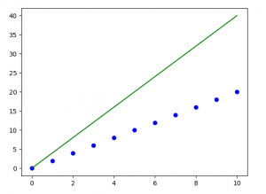
#original best-fit line
Y_pred = regressor.predict()
regressor.plot_best_fit(Y_pred, 'Initial Best Fit Line')
while 1:
Y_pred = regressor.predict()
cost = regressor.compute_cost(Y_pred)
costs.append(cost)
regressor.update_coeffs(learning_rate)
iterations += 1
if iterations % steps == 0:
print(iterations, "epochs elapsed")
print("Current accuracy is :",
regressor.get_current_accuracy(Y_pred))
stop = input("Do you want to stop (y/*)??")
if stop == "y":
break
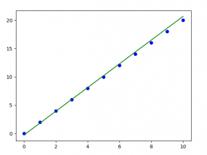
#final best-fit line
regressor.plot_best_fit(Y_pred, 'Final Best Fit Line')
#plot to verify cost function decreases
h = plt.figure('Verification')
plt.plot(range(iterations), costs, color='b')
h.show()
# if user wants to predict using the regressor:
regressor.predict([i for i in range(10)])
if __name__ == '__main__':
main()输出:
注意:梯度下降有时也使用正则化来实现。