Python – 统计中的逆高斯分布

scipy.stats.invgauss()是一个倒置高斯连续随机变量。它作为rv_continuous 类的实例继承自泛型方法。它使用特定于此特定发行版的详细信息来完成方法。

参数 ：

a : shape parameter
c : special case of gengauss. Default equals to c = -1

代码#1：创建逆高斯连续随机变量

# importing library
from scipy.stats import invgauss   
     
numargs = invgauss.numargs 
[a, b] = [0.7, 0.4] * numargs 
rv = invgauss (a, b) 
     
print ("RV : \n", rv)  

输出 ：

RV : 
 scipy.stats._distn_infrastructure.rv_frozen object at 0x1a220d7bd0

代码#2：逆高斯连续变量和概率分布

import numpy as np 
quantile = np.arange (0.01, 1) 
      
# Random Variates 
R = invgauss.ppf(0.01, a) 
print ("Random Variates : \n", R) 
     
# PDF 
R = invgauss.pdf(invgauss.ppf(0.01, a), a) 
print ("\nProbability Distribution : \n", R) 

输出 ：

Random Variates : 
 0.25801533159920903

Probability Distribution : 
 0.15984442779701688

代码#3：图形表示。

import numpy as np 
import matplotlib.pyplot as plt 
     
distribution = np.linspace(0, np.minimum(rv.dist.b, 3)) 
print("Distribution : \n", distribution) 
     
plot = plt.plot(distribution, rv.pdf(distribution)) 

输出 ：

Distribution : 
 [0.         0.06122449 0.12244898 0.18367347 0.24489796 0.30612245
 0.36734694 0.42857143 0.48979592 0.55102041 0.6122449  0.67346939
 0.73469388 0.79591837 0.85714286 0.91836735 0.97959184 1.04081633
 1.10204082 1.16326531 1.2244898  1.28571429 1.34693878 1.40816327
 1.46938776 1.53061224 1.59183673 1.65306122 1.71428571 1.7755102
 1.83673469 1.89795918 1.95918367 2.02040816 2.08163265 2.14285714
 2.20408163 2.26530612 2.32653061 2.3877551  2.44897959 2.51020408
 2.57142857 2.63265306 2.69387755 2.75510204 2.81632653 2.87755102
 2.93877551 3.        ]

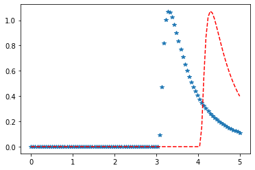
代码#4：改变位置参数

import matplotlib.pyplot as plt 
import numpy as np 
     
x = np.linspace(0, 5, 100) 
     
# Varying positional arguments 
y1 = invgauss .pdf(x, 1, 3) 
y2 = invgauss .pdf(x, 1, 4) 
plt.plot(x, y1, "*", x, y2, "r--") 

输出 ：