在 PyTorch 中实现深度自动编码器进行图像重建

由于互联网上的数据量惊人，工业界和学术界的研究人员和科学家一直在努力开发比当前最先进的方法更有效、更可靠的数据传输模式。自编码器是最近发现的用于此类任务的关键元素之一，其结构简单直观。

概括地说，一旦自编码器被训练，编码器的权重就可以发送到发送端，解码器的权重可以发送到接收端。这样，发送方可以以编码格式发送数据（从而节省时间和金钱），而接收方可以以更少的检修来接收数据。本文将探讨自动编码器的一个有趣应用，该应用可用于使用Python中的 Pytorch 框架在著名的 MNIST 数字数据集上进行图像重建。

自编码器

如下图所示，一个非常基本的自动编码器由两个主要部分组成：

1. 编码器和，
2. 解码器

通过一系列层，编码器获取输入并将高维数据转换为相同值的潜在低维表示。解码器采用这种潜在表示并输出重建的数据。

为了更深入地理解该理论，鼓励读者阅读以下文章：ML |自动编码器

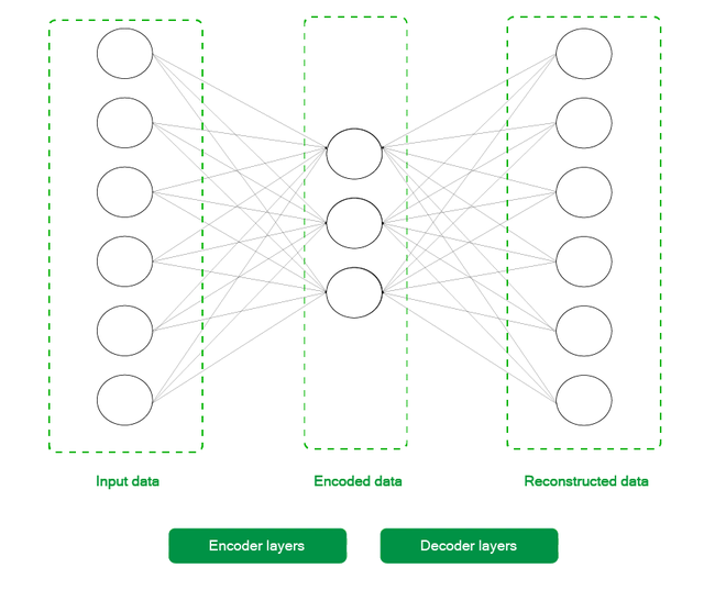
一个基本的 2 层自动编码器

安装：

除了Numpy和Matplotlib等常用库外，本文只需要Pytorch工具链中的torch和torchvision库。您可以使用以下命令来获取所有这些库。

pip3 install torch torchvision torchaudio numpy matplotlib

现在进入最有趣的部分，代码。本文假设您基本熟悉PyTorch工作流及其各种实用程序，如数据加载器、数据集和张量转换。为了快速复习这些概念，鼓励读者阅读以下文章：

• 使用 PyTorch 使用验证训练神经网络
• PyTorch 入门

代码分为 5 个不同的步骤，以实现更好的材料流动，并按顺序执行以确保正常工作。每个步骤的开头也有一些要点，可以帮助读者更好地理解该步骤的代码。

分步实施：

步骤 1：从训练集中加载数据并打印一些样本图像。

• 初始化变换：首先，我们初始化将应用于获得的数据集中每个条目的变换。由于张量是 Pytorch 功能的内部，我们首先将每个项目转换为张量并将它们归一化以将像素值限制在 0 和 1 之间。这样做是为了使优化过程更容易和更快。
• 下载数据集：然后，我们使用torchvision.datasets实用程序下载数据集，并将其存储在我们本地机器上的文件夹./MNIST/train和./MNIST/test中，用于训练集和测试集。我们还将这些数据集转换为批大小等于 256 的数据加载器，以加快学习速度。鼓励读者尝试这些值并期待一致的结果。
• 绘制数据集：最后，我们从数据集中随机打印出 25 张图像，以更好地查看我们正在处理的数据。

代码：

Python

# Importing the necessary libraries
import numpy as np
import matplotlib.pyplot as plt
import torchvision
import torch
plt.rcParams['figure.figsize'] = 15, 10
  
# Initializing the transform for the dataset
transform = torchvision.transforms.Compose([
    torchvision.transforms.ToTensor(),
    torchvision.transforms.Normalize((0.5), (0.5))
])
  
# Downloading the MNIST dataset
train_dataset = torchvision.datasets.MNIST(
    root="./MNIST/train", train=True,
    transform=torchvision.transforms.ToTensor(),
    download=True)
  
test_dataset = torchvision.datasets.MNIST(
    root="./MNIST/test", train=False,
    transform=torchvision.transforms.ToTensor(),
    download=True)
  
# Creating Dataloaders from the
# training and testing dataset
train_loader = torch.utils.data.DataLoader(
    train_dataset, batch_size=256)
test_loader = torch.utils.data.DataLoader(
    test_dataset, batch_size=256)
  
# Printing 25 random images from the training dataset
random_samples = np.random.randint(
    1, len(train_dataset), (25))
  
for idx in range(random_samples.shape[0]):
    plt.subplot(5, 5, idx + 1)
    plt.imshow(train_dataset[idx][0][0].numpy(), cmap='gray')
    plt.title(train_dataset[idx][1])
    plt.axis('off')
  
plt.tight_layout()
plt.show()

输出：

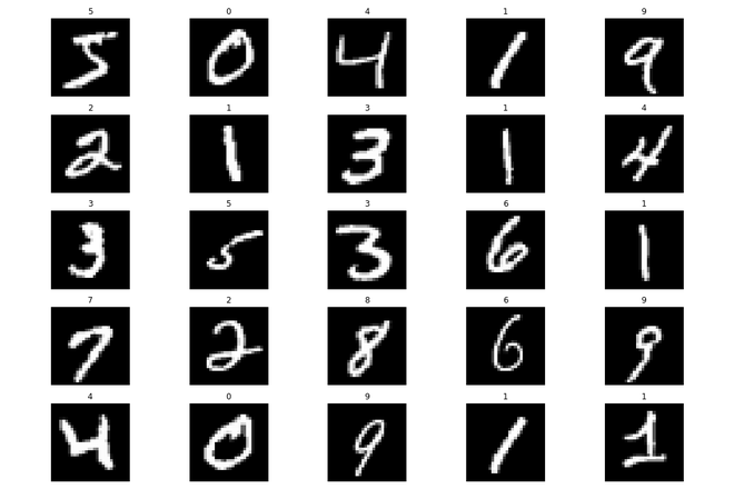
训练集中的随机样本

第 2 步：初始化 Deep Autoencoder 模型和其他超参数

在这一步中，我们初始化DeepAutoencoder类，它是torch.nn.Module的子类。这为我们抽象了很多样板代码，现在我们可以专注于构建我们的模型架构如下：

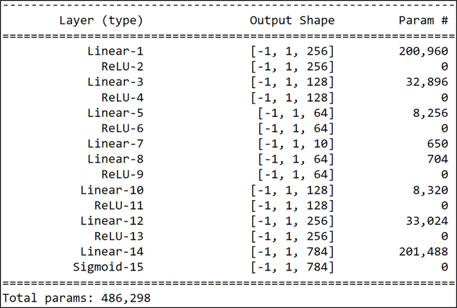
模型架构

如上所述，编码器层形成了网络的前半部分，即从 Linear-1 到 Linear-7 ，而解码器形成了从 Linear-10 到 Sigmoid-15 的另一半。我们使用了torch.nn.Sequential实用程序将编码器和解码器彼此分开。这样做是为了更好地理解模型的架构。之后，我们初始化一些模型超参数，以便在学习过程中使用均方误差损失和 Adam 优化器对 100 个时期进行训练。

Python

# Creating a DeepAutoencoder class
class DeepAutoencoder(torch.nn.Module):
    def __init__(self):
        super().__init__()        
        self.encoder = torch.nn.Sequential(
            torch.nn.Linear(28 * 28, 256),
            torch.nn.ReLU(),
            torch.nn.Linear(256, 128),
            torch.nn.ReLU(),
            torch.nn.Linear(128, 64),
            torch.nn.ReLU(),
            torch.nn.Linear(64, 10)
        )
          
        self.decoder = torch.nn.Sequential(
            torch.nn.Linear(10, 64),
            torch.nn.ReLU(),
            torch.nn.Linear(64, 128),
            torch.nn.ReLU(),
            torch.nn.Linear(128, 256),
            torch.nn.ReLU(),
            torch.nn.Linear(256, 28 * 28),
            torch.nn.Sigmoid()
        )
  
    def forward(self, x):
        encoded = self.encoder(x)
        decoded = self.decoder(encoded)
        return decoded
  
# Instantiating the model and hyperparameters
model = DeepAutoencoder()
criterion = torch.nn.MSELoss()
num_epochs = 100
optimizer = torch.optim.Adam(model.parameters(), lr=1e-3)

第 3 步：训练循环

训练循环迭代 100 个时期并执行以下操作：

• 迭代每个批次并计算输出图像和原始图像（即输出）之间的损失。
• 平均每个批次的损失并存储每个时期的图像及其输出。

循环结束后，我们绘制出训练损失以更好地理解训练过程。如我们所见，每个连续 epoch 的损失都会减少，因此可以认为训练是成功的。

Python

# List that will store the training loss
train_loss = []
  
# Dictionary that will store the
# different images and outputs for 
# various epochs
outputs = {}
  
batch_size = len(train_loader)
  
# Training loop starts
for epoch in range(num_epochs):
        
    # Initializing variable for storing 
    # loss
    running_loss = 0
      
    # Iterating over the training dataset
    for batch in train_loader:
            
        # Loading image(s) and
        # reshaping it into a 1-d vector
        img, _ = batch  
        img = img.reshape(-1, 28*28)
          
        # Generating output
        out = model(img)
          
        # Calculating loss
        loss = criterion(out, img)
          
        # Updating weights according
        # to the calculated loss
        optimizer.zero_grad()
        loss.backward()
        optimizer.step()
          
        # Incrementing loss
        running_loss += loss.item()
      
    # Averaging out loss over entire batch
    running_loss /= batch_size
    train_loss.append(running_loss)
      
    # Storing useful images and
    # reconstructed outputs for the last batch
    outputs[epoch+1] = {'img': img, 'out': out}
  
  
# Plotting the training loss
plt.plot(range(1,num_epochs+1),train_loss)
plt.xlabel("Number of epochs")
plt.ylabel("Training Loss")
plt.show()

输出：

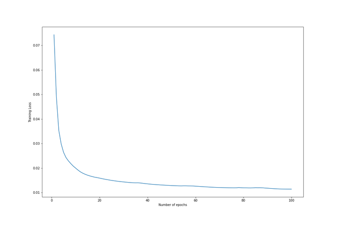
训练损失 vs. Epochs

第 4 步：可视化重建

这个项目最好的部分是读者可以可视化每个 epoch 的重建并理解模型的迭代学习。

• 我们首先绘制出 epochs = [1, 5, 10, 50, 100] 的前 5 个重建（或输出图像）。
• 然后我们还在底部绘制相应的原始图像以进行比较。

我们可以看到每个时期的重建如何改进，并在最后一个时期非常接近原始时期。

Python

# Plotting is done on a 7x5 subplot
# Plotting the reconstructed images
  
# Initializing subplot counter
counter = 1
  
# Plotting reconstructions
# for epochs = [1, 5, 10, 50, 100]
epochs_list = [1, 5, 10, 50, 100]
  
# Iterating over specified epochs
for val in epochs_list:
    
      # Extracting recorded information
    temp = outputs[val]['out'].detach().numpy()
    title_text = f"Epoch = {val}"
      
    # Plotting first five images of the last batch
    for idx in range(5):
        plt.subplot(7, 5, counter)
        plt.title(title_text)
        plt.imshow(temp[idx].reshape(28,28), cmap= 'gray')
        plt.axis('off')
          
        # Incrementing the subplot counter
        counter+=1
  
# Plotting original images
  
# Iterating over first five
# images of the last batch
for idx in range(5):
      
    # Obtaining image from the dictionary
    val = outputs[10]['img']
      
    # Plotting image
    plt.subplot(7,5,counter)
    plt.imshow(val[idx].reshape(28, 28),
               cmap = 'gray')
    plt.title("Original Image")
    plt.axis('off')
      
    # Incrementing subplot counter
    counter+=1
  
plt.tight_layout()
plt.show()

输出：

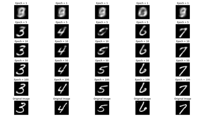
从训练过程中收集的数据中可视化重建

第 5 步：在测试集上检查性能。

机器学习的良好做法是检查模型在测试集上的性能。为此，我们执行以下步骤：

• 为最后一批测试集生成输出。
• 绘制前 10 个输出和相应的原始图像进行比较。

正如我们所看到的，在这个测试集上的重建也很出色，完成了管道。

Python

# Dictionary that will store the different
# images and outputs for various epochs
outputs = {}
  
# Extracting the last batch from the test 
# dataset
img, _ = list(test_loader)[-1]
  
# Reshaping into 1d vector
img = img.reshape(-1, 28 * 28)
  
# Generating output for the obtained
# batch
out = model(img)
  
# Storing information in dictionary
outputs['img'] = img
outputs['out'] = out
  
# Plotting reconstructed images
# Initializing subplot counter
counter = 1
val = outputs['out'].detach().numpy()
  
# Plotting first 10 images of the batch
for idx in range(10):
    plt.subplot(2, 10, counter)
    plt.title("Reconstructed \n image")
    plt.imshow(val[idx].reshape(28, 28), cmap='gray')
    plt.axis('off')
  
    # Incrementing subplot counter
    counter += 1
  
# Plotting original images
  
# Plotting first 10 images
for idx in range(10):
    val = outputs['img']
    plt.subplot(2, 10, counter)
    plt.imshow(val[idx].reshape(28, 28), cmap='gray')
    plt.title("Original Image")
    plt.axis('off')
  
    # Incrementing subplot counter
    counter += 1
  
plt.tight_layout()
plt.show()

输出：

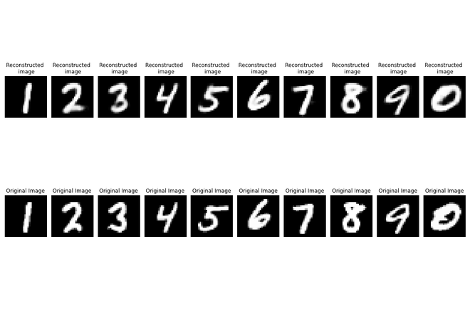
在测试集上验证性能

结论：

自编码器正迅速成为机器学习中最令人兴奋的研究领域之一。本文介绍了用于图像重建的深度自动编码器的 Pytorch 实现。鼓励读者尝试使用网络架构和超参数来提高重建质量和损失值。