在 PyTorch 中实现自动编码器

自编码器是一种神经网络，它生成给定输入的“n 层”编码，并尝试使用生成的代码重建输入。这种神经网络架构分为编码器结构、解码器结构和潜在空间，也称为“瓶颈”。为了学习输入的数据表示，网络使用无监督数据进行训练。这些压缩的数据表示经过解码过程，其中输入被重建。自编码器是一种对恒等函数建模的回归任务。

编码器结构

该结构包括传统的前馈神经网络，其结构化为预测输入数据的潜在视图表示。它由以下给出：

$h_z = f_e(g_e(x_i))$

在哪里$g_e$表示隐藏层 1， $f_e$表示隐藏层 2， $x_i$表示自编码器的输入，h 表示输入的低维数据空间

解码器结构

这种结构包括一个前馈神经网络，但数据的维度按照编码器层的顺序增加，用于预测输入。它由以下给出：

$\bar x = g_d(f_d(h_z))$

在哪里$f_d$表示隐藏层 1， $g_d$表示隐藏层 2， $h_z$表示由编码器结构生成的低维数据空间和$\bar x$表示重建的输入。

潜在空间结构

这是模型输入的数据表示或低级压缩表示。解码器结构使用这种低维形式的数据来重构输入。它由$h_z$

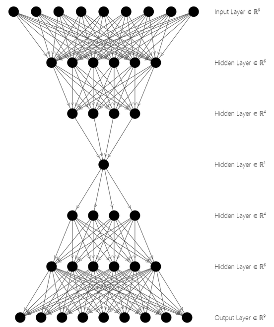
自编码器架构

上图中，上面三层代表Encoder Block，下面三层代表Decoder Block。潜在状态空间位于架构的中间$R^1$ .自编码器用于图像压缩、特征提取、降维等。现在让我们看看实现。

需要的模块

• torch：这个Python包提供了基于 autograd 系统的高级张量计算和深度神经网络。

pip install torch

• torchvision：该模块由广泛的数据库、图像架构和计算机视觉转换组成

pip install torchvision

Pytorch中Autoencoder的实现

步骤 1：导入模块

我们将使用 Torch 包中的 torch.optim 和 torch.nn 模块，以及 torchvision 包中的数据集和转换。在本文中，我们将使用流行的 MNIST 数据集，其中包含 0 到 9 之间的手写单个数字的灰度图像。

Python3

import torch
from torchvision import datasets
from torchvision import transforms
import matplotlib.pyplot as plt

第 2 步：加载数据集

此代码段使用 DataLoader 模块将 MNIST 数据集加载到加载器中。数据集被下载并转换为图像张量。使用 DataLoader 模块，张量被加载并准备好使用。数据集加载时启用了 Shuffling，批大小为 64。

蟒蛇3

# Transforms images to a PyTorch Tensor
tensor_transform = transforms.ToTensor()
  
# Download the MNIST Dataset
dataset = datasets.MNIST(root = "./data",
                         train = True,
                         download = True,
                         transform = tensor_transform)
  
# DataLoader is used to load the dataset 
# for training
loader = torch.utils.data.DataLoader(dataset = dataset,
                                     batch_size = 32,
                                     shuffle = True)

第 3 步：创建自动编码器类

在此编码片段中，编码器部分按以下顺序减少数据的维数：

28*28 = 784 ==> 128 ==> 64 ==> 36 ==> 18 ==> 9

其中输入节点的数量为 784，在潜在空间中被编码为 9 个节点。而在解码器部分，数据的维数线性增加到原始输入大小，以重建输入。

9 ==> 18 ==> 36 ==> 64 ==> 128 ==> 784 ==> 28*28 = 784

其中输入是 9 节点潜在空间表示，输出是 28*28 重构输入。

编码器从线性层中的 28*28 个节点开始，然后是 ReLU 层，直到维数减少到 9 个节点。解密器使用这 9 个数据表示通过使用编码器架构的逆来恢复原始图像。解密器架构使用 Sigmoid 层仅将值设置在 0 和 1 之间。

蟒蛇3

# Creating a PyTorch class
# 28*28 ==> 9 ==> 28*28
class AE(torch.nn.Module):
    def __init__(self):
        super().__init__()
          
        # Building an linear encoder with Linear
        # layer followed by Relu activation function
        # 784 ==> 9
        self.encoder = torch.nn.Sequential(
            torch.nn.Linear(28 * 28, 128),
            torch.nn.ReLU(),
            torch.nn.Linear(128, 64),
            torch.nn.ReLU(),
            torch.nn.Linear(64, 36),
            torch.nn.ReLU(),
            torch.nn.Linear(36, 18),
            torch.nn.ReLU(),
            torch.nn.Linear(18, 9)
        )
          
        # Building an linear decoder with Linear
        # layer followed by Relu activation function
        # The Sigmoid activation function
        # outputs the value between 0 and 1
        # 9 ==> 784
        self.decoder = torch.nn.Sequential(
            torch.nn.Linear(9, 18),
            torch.nn.ReLU(),
            torch.nn.Linear(18, 36),
            torch.nn.ReLU(),
            torch.nn.Linear(36, 64),
            torch.nn.ReLU(),
            torch.nn.Linear(64, 128),
            torch.nn.ReLU(),
            torch.nn.Linear(128, 28 * 28),
            torch.nn.Sigmoid()
        )
  
    def forward(self, x):
        encoded = self.encoder(x)
        decoded = self.decoder(encoded)
        return decoded

第 4 步：初始化模型

我们使用均方误差函数验证模型，我们使用 Adam 优化器，其学习率为 0.1，权重衰减为$10^{-8}$

蟒蛇3

# Model Initialization
model = AE()
  
# Validation using MSE Loss function
loss_function = torch.nn.MSELoss()
  
# Using an Adam Optimizer with lr = 0.1
optimizer = torch.optim.Adam(model.parameters(),
                             lr = 1e-1,
                             weight_decay = 1e-8)

第 5 步：创建输出生成

每个时期的输出是通过作为参数传递到 Model() 类中来计算的，最终的张量存储在输出列表中。图像进入 (-1, 784) 并作为参数传递给 Autoencoder 类，后者又返回重建的图像。损失函数使用 MSELoss函数计算并绘制。在优化器中，使用 zero_grad() 将初始梯度值设置为零。 loss.backward() 计算梯度值并存储。使用 step()函数更新优化器。

输出列表中的原始图像和重建图像被分离并转换为 NumPy 数组以绘制图像。

注意：此代码段需要 15 到 20 分钟才能执行，具体取决于处理器类型。初始化 epoch = 1，以获得快速结果。使用 GPU/TPU 运行时进行更快的计算。

蟒蛇3

epochs = 20
outputs = []
losses = []
for epoch in range(epochs):
    for (image, _) in loader:
        
      # Reshaping the image to (-1, 784)
      image = image.reshape(-1, 28*28)
        
      # Output of Autoencoder
      reconstructed = model(image)
        
      # Calculating the loss function
      loss = loss_function(reconstructed, image)
        
      # The gradients are set to zero,
      # the the gradient is computed and stored.
      # .step() performs parameter update
      optimizer.zero_grad()
      loss.backward()
      optimizer.step()
        
      # Storing the losses in a list for plotting
      losses.append(loss)
    outputs.append((epochs, image, reconstructed))
  
# Defining the Plot Style
plt.style.use('fivethirtyeight')
plt.xlabel('Iterations')
plt.ylabel('Loss')
  
# Plotting the last 100 values
plt.plot(losses[-100:])

输出：

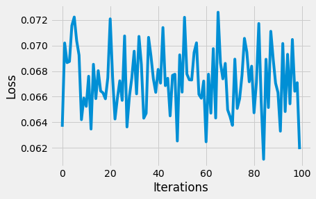
损失函数图

第 6 步：输入/重构输入到/来自自动编码器

第一个输入图像数组和第一个重建的输入图像数组已使用 plt.imshow() 绘制。

蟒蛇3

for i, item in enumerate(image):
    
  # Reshape the array for plotting
  item = item.reshape(-1, 28, 28)
  plt.imshow(item[0])
  
for i, item in enumerate(reconstructed):
  item = item.reshape(-1, 28, 28)
  plt.imshow(item[0])

输出：

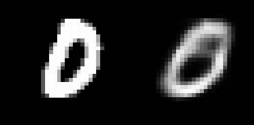
示例图 1：输入图像（左）和重建输入（右）

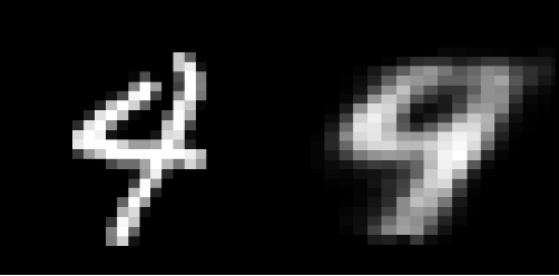
示例图 2：输入图像（左）和重建输入（右）

虽然重建的图片看起来足够了，但它们非常有颗粒感。为了增强这一结果，可以添加额外的层和/或神经元，或者可以在卷积神经网络架构上构建自动编码器模型。对于降维，自编码器非常有用。但是，它也可能用于数据去噪和理解数据集的传播。