Python深度学习-实现

📌 相关文章

📜 Python深度学习-实现

📅 最后修改于: 2020-12-13 14:29:05 🧑 作者: Mango

在实施深度学习的过程中，我们的目标是预测特定银行的客户流失或搅动数据-哪些客户可能会退出该银行服务。使用的数据集相对较小，包含10000行和14列。我们正在使用Anaconda发行版以及Theano，TensorFlow和Keras之类的框架。 Keras是建立在Tensorflow和Theano它函数其后端的顶部。

# Artificial Neural Network
# Installing Theano
pip install --upgrade theano

# Installing Tensorflow
pip install –upgrade tensorflow

# Installing Keras
pip install --upgrade keras

步骤1：资料预处理

In[]:

# Importing the libraries
   import numpy as np
   import matplotlib.pyplot as plt
   import pandas as pd
 
# Importing the database
   dataset = pd.read_csv('Churn_Modelling.csv')

第2步

我们创建数据集特征和目标变量的矩阵，该变量位于第14列，标记为“已退出”。

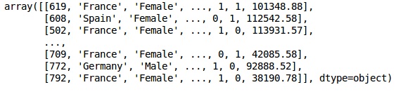
数据的初始外观如下所示-

In[]:
X = dataset.iloc[:, 3:13].values
Y = dataset.iloc[:, 13].values
X

输出

步进输出

第三步

输出

array([1, 0, 1, ..., 1, 1, 0], dtype = int64)

第4步

通过编码字符串变量，我们使分析更加简单。我们正在使用ScikitLearn函数“ LabelEncoder”自动对列中值在0到n_classes-1之间的不同标签进行编码。

from sklearn.preprocessing import LabelEncoder, OneHotEncoder
labelencoder_X_1 = LabelEncoder() 
X[:,1] = labelencoder_X_1.fit_transform(X[:,1]) 
labelencoder_X_2 = LabelEncoder() 
X[:, 2] = labelencoder_X_2.fit_transform(X[:, 2])
X

输出

第四步输出

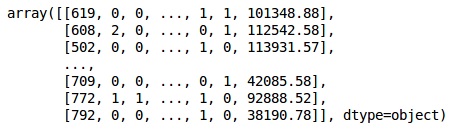
在上面的输出中，国家名称被0、1和2替换；而将男性和女性分别替换为0和1。

第5步

标记编码数据

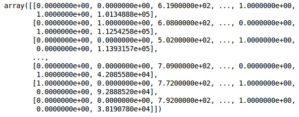
我们使用相同的ScikitLearn库和另一个称为OneHotEncoder的函数来传递列号，从而创建一个虚拟变量。

onehotencoder = OneHotEncoder(categorical features = [1])
X = onehotencoder.fit_transform(X).toarray()
X = X[:, 1:]
X

现在，前两列代表国家，第四列代表性别。

输出

Step5输出

我们始终将数据分为培训和测试部分；我们在训练数据上训练模型，然后在测试数据上检查模型的准确性，这有助于评估模型的效率。

第6步

我们正在使用ScikitLearn的train_test_split函数将数据分为训练集和测试集。我们将火车与测试的比率保持为80:20。

#Splitting the dataset into the Training set and the Test Set
from sklearn.model_selection import train_test_split
X_train, X_test, y_train, y_test = train_test_split(X, y, test_size = 0.2)

有些变量的值是数千，而有些变量的值是十或一。我们缩放数据，以便它们更具代表性。

步骤7

在此代码中，我们使用StandardScaler函数拟合和转换训练数据。我们将缩放比例标准化，以便我们使用相同的拟合方法来转换/缩放测试数据。

# Feature Scaling

fromsklearn.preprocessing import StandardScaler 
sc = StandardScaler() 
X_train = sc.fit_transform(X_train) 
X_test = sc.transform(X_test)

输出

step7输出

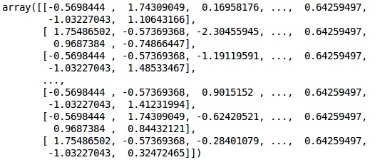
现在，数据已正确缩放。最后，我们完成了数据预处理。现在，我们将从模型开始。

步骤8

我们在此处导入所需的模块。我们需要用于初始化神经网络的顺序模块和需要添加隐藏层的密集模块。

# Importing the Keras libraries and packages 
import keras 
from keras.models import Sequential 
from keras.layers import Dense

步骤9

我们将模型命名为“分类器”，因为我们的目的是对客户流失进行分类。然后，我们使用顺序模块进行初始化。

#Initializing Neural Network 
classifier = Sequential()

第10步

我们使用稠密函数将隐藏的层一一添加。在下面的代码中，我们将看到许多参数。

我们的第一个参数是output_dim 。这是我们添加到此层的节点数。 init是随机渐变体面的初始化。在神经网络中，我们为每个节点分配权重。初始化时，权重应接近零，我们使用统一函数随机初始化权重。由于模型不知道输入变量的数量，因此仅在第一层需要input_dim参数。此处，输入变量的总数为11。在第二层中，模型会自动从第一隐藏层中知道输入变量的数目。

执行以下代码行以添加输入层和第一个隐藏层-

classifier.add(Dense(units = 6, kernel_initializer = 'uniform', 
activation = 'relu', input_dim = 11))

执行以下代码行以添加第二个隐藏层-

classifier.add(Dense(units = 6, kernel_initializer = 'uniform', 
activation = 'relu'))

执行以下代码行添加输出层-

classifier.add(Dense(units = 1, kernel_initializer = 'uniform', 
activation = 'sigmoid'))

步骤11

编译神经网络

到目前为止，我们已经在分类器中添加了多层。现在，我们将使用compile方法对其进行编译。在最终编译控件中添加的参数完善了神经网络。因此，在此步骤中我们需要小心。

这是对参数的简要说明。

第一个参数是Optimizer，这是一种用于找到最佳权重集的算法。该算法称为随机梯度下降(SGD) 。在这里，我们使用几种类型中的一种，称为“亚当优化器”。 SGD取决于损失，因此我们的第二个参数是损失。如果我们的因变量是二进制，则使用称为‘binary_crossentropy’的对数损失函数，如果我们的因变量在输出中具有两个以上的类别，则使用‘categorical_crossentropy’ 。我们希望基于准确性来改善神经网络的性能，因此我们添加了度量作为准确性。

# Compiling Neural Network 
classifier.compile(optimizer = 'adam', loss = 'binary_crossentropy', metrics = ['accuracy'])

步骤12

在此步骤中需要执行许多代码。

将ANN拟合到训练集

现在，我们在训练数据上训练模型。我们使用拟合方法来拟合我们的模型。我们还优化权重以提高模型效率。为此，我们必须更新权重。批次大小是观察值的数量，之后我们将更新权重。时代是迭代的总数。批次大小和时期的值是通过反复试验方法选择的。

classifier.fit(X_train, y_train, batch_size = 10, epochs = 50)

进行预测并评估模型

# Predicting the Test set results
y_pred = classifier.predict(X_test)
y_pred = (y_pred > 0.5)

预测一个新的观察

# Predicting a single new observation
"""Our goal is to predict if the customer with the following data will leave the bank:
Geography: Spain
Credit Score: 500
Gender: Female
Age: 40
Tenure: 3
Balance: 50000
Number of Products: 2
Has Credit Card: Yes
Is Active Member: Yes

步骤13

预测测试结果

预测结果将给您客户离开公司的可能性。我们将那个概率转换为二进制0和1。

# Predicting the Test set results 
y_pred = classifier.predict(X_test) 
y_pred = (y_pred > 0.5)

new_prediction = classifier.predict(sc.transform
(np.array([[0.0, 0, 500, 1, 40, 3, 50000, 2, 1, 1, 40000]])))
new_prediction = (new_prediction > 0.5)

步骤14

这是我们评估模型性能的最后一步。我们已经有了原始结果，因此可以构建混淆矩阵来检查模型的准确性。

制作混乱矩阵

from sklearn.metrics import confusion_matrix
cm = confusion_matrix(y_test, y_pred)
print (cm)

输出

loss: 0.3384 acc: 0.8605
[ [1541 54]
[230 175] ]

根据混淆矩阵，我们模型的精度可以计算为-

Accuracy = 1541+175/2000=0.858

我们达到了85.8％的准确度，这是很好的。

正向传播算法

在本节中，我们将学习如何为简单的神经网络编写代码以进行正向传播(预测)-

正向传播算法

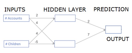
每个数据点都是一个客户。第一个输入是他们有多少个帐户，第二个输入是他们有多少个孩子。该模型将预测用户在明年进行的交易次数。

输入数据被预加载为输入数据，权重在称为权重的字典中。隐藏层中第一个节点的权重数组以权重[‘node_0’]表示，隐藏层中第二个节点的权重数组分别以权重[‘node_1’]表示。

馈入输出节点的权重可用权重提供。

整流线性激活函数

“激活函数”是在每个节点上起作用的函数。它将节点的输入转换为某些输出。

整流的线性激活函数(称为ReLU )广泛用于非常高性能的网络中。此函数将一个数字作为输入，如果输入为负，则返回0，如果输入为正，则返回输入。

这是一些例子-

relu(4)= 4
relu(-2)= 0

我们填写relu()函数的定义-

我们使用max()函数来计算relu()的输出值。
我们将relu()函数应用于node_0_input来计算node_0_output。
我们将relu()函数应用于node_1_input以计算node_1_output。

import numpy as np
input_data = np.array([-1, 2])
weights = {
   'node_0': np.array([3, 3]),
   'node_1': np.array([1, 5]),
   'output': np.array([2, -1])
}
node_0_input = (input_data * weights['node_0']).sum()
node_0_output = np.tanh(node_0_input)
node_1_input = (input_data * weights['node_1']).sum()
node_1_output = np.tanh(node_1_input)
hidden_layer_output = np.array(node_0_output, node_1_output)
output =(hidden_layer_output * weights['output']).sum()
print(output)

def relu(input):
   '''Define your relu activation function here'''
   # Calculate the value for the output of the relu function: output
   output = max(input,0)
      # Return the value just calculated
   return(output)
# Calculate node 0 value: node_0_output
node_0_input = (input_data * weights['node_0']).sum()
node_0_output = relu(node_0_input)

# Calculate node 1 value: node_1_output
node_1_input = (input_data * weights['node_1']).sum()
node_1_output = relu(node_1_input)

# Put node values into array: hidden_layer_outputs
hidden_layer_outputs = np.array([node_0_output, node_1_output])

# Calculate model output (do not apply relu)
odel_output = (hidden_layer_outputs * weights['output']).sum()
print(model_output)# Print model output

输出

0.9950547536867305
-3

将网络应用于许多观测/数据行

在本节中，我们将学习如何定义一个名为predict_with_network()的函数。此函数将针对来自上方网络的多个数据观测值生成预测，作为输入数据。使用上述网络中给出的权重。还使用了relu()函数定义。

让我们定义一个名为predict_with_network()的函数，该函数接受两个参数(input_data_row和weights)，并从网络返回一个预测作为输出。

我们计算每个节点的输入和输出值，并将它们存储为：node_0_input，node_0_output，node_1_input和node_1_output。

为了计算节点的输入值，我们将相关数组相乘并计算它们的总和。

为了计算节点的输出值，我们将relu()函数应用于节点的输入值。我们使用’for循环’遍历input_data-

我们还使用predict_with_network()为input_data-input_data_row的每一行生成预测。我们还将每个预测附加到结果中。

# Define predict_with_network()
def predict_with_network(input_data_row, weights):
   # Calculate node 0 value
   node_0_input = (input_data_row * weights['node_0']).sum()
   node_0_output = relu(node_0_input)
   
   # Calculate node 1 value
   node_1_input = (input_data_row * weights['node_1']).sum()
   node_1_output = relu(node_1_input)
   
   # Put node values into array: hidden_layer_outputs
   hidden_layer_outputs = np.array([node_0_output, node_1_output])
   
   # Calculate model output
   input_to_final_layer = (hidden_layer_outputs*weights['output']).sum()
   model_output = relu(input_to_final_layer)
# Return model output
   return(model_output)

# Create empty list to store prediction results
results = []
for input_data_row in input_data:
   # Append prediction to results
   results.append(predict_with_network(input_data_row, weights))
print(results)# Print results

输出

[0, 12]

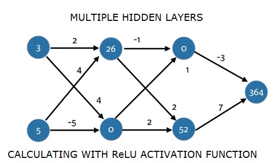
在这里，我们使用了relu函数，其中relu(26)= 26和relu(-13)= 0等等。

深度多层神经网络

在这里，我们正在编写代码以对具有两个隐藏层的神经网络进行正向传播。每个隐藏层都有两个节点。输入数据已预加载为input_data 。第一隐藏层中的节点称为node_0_0和node_0_1。

它们的权重分别预加载为weights [‘node_0_0’]和weights [‘node_0_1’]。

第二隐藏层中的节点称为node_1_0和node_1_1 。它们的权重分别预加载为weights [‘node_1_0’]和weights [‘node_1_1’] 。

然后，我们使用预加载为weights [‘output’]的权重从隐藏节点创建模型输出。

深多层

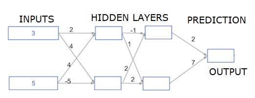
我们使用权重weights [‘node_0_0’]和给定的input_data来计算node_0_0_input。然后应用relu()函数获取node_0_0_output。

我们对node_0_1_input进行与上述相同的操作，以获取node_0_1_output。

我们使用权重weights [‘node_1_0’]和第一个隐藏层的输出-hidden_0_outputs来计算node_1_0_input。然后，我们应用relu()函数来获取node_1_0_output。

我们对node_1_1_input进行与上述相同的操作，以获取node_1_1_output。

我们使用weights [‘output’]和第二个隐藏层hidden_1_outputs数组的输出来计算model_output。我们不将relu()函数应用于此输出。

多隐藏层

import numpy as np
input_data = np.array([3, 5])
weights = {
   'node_0_0': np.array([2, 4]),
   'node_0_1': np.array([4, -5]),
   'node_1_0': np.array([-1, 1]),
   'node_1_1': np.array([2, 2]),
   'output': np.array([2, 7])
}
def predict_with_network(input_data):
   # Calculate node 0 in the first hidden layer
   node_0_0_input = (input_data * weights['node_0_0']).sum()
   node_0_0_output = relu(node_0_0_input)
   
   # Calculate node 1 in the first hidden layer
   node_0_1_input = (input_data*weights['node_0_1']).sum()
   node_0_1_output = relu(node_0_1_input)
   
   # Put node values into array: hidden_0_outputs
   hidden_0_outputs = np.array([node_0_0_output, node_0_1_output])
   
   # Calculate node 0 in the second hidden layer
   node_1_0_input = (hidden_0_outputs*weights['node_1_0']).sum()
   node_1_0_output = relu(node_1_0_input)
   
   # Calculate node 1 in the second hidden layer
   node_1_1_input = (hidden_0_outputs*weights['node_1_1']).sum()
   node_1_1_output = relu(node_1_1_input)
   
   # Put node values into array: hidden_1_outputs
   hidden_1_outputs = np.array([node_1_0_output, node_1_1_output])
   
   # Calculate model output: model_output
   model_output = (hidden_1_outputs*weights['output']).sum()
      # Return model_output
   return(model_output)
output = predict_with_network(input_data)
print(output)