毫升 |非线性支持向量机

先决条件：使用 SVM 对数据进行分类

在线性支持向量机中，这两个类是线性可分的，即一条直线能够对这两个类进行分类。但是想象一下，如果你有三个类，显然它们不会是线性可分的。因此，在处理类不是线性可分的这类数据时，非线性 SVM 会派上用场。

我们将讨论非线性核，即RBF 核（径向基函数核）。所以，这个内核基本上所做的就是尝试将给定的数据转换为几乎线性可分的数据。

让我们考虑仅使用 4 个特征中的 2 个（花瓣长度和花瓣宽度）绘制的 IRIS 数据集的示例。

以下是相同的散点图：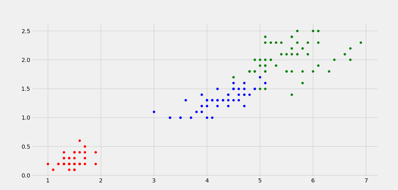

很明显，这些类不是线性可分的。下面是非线性 SVM 的等值线图，它使用 RBF 核成功地对 IRIS 数据集进行了分类。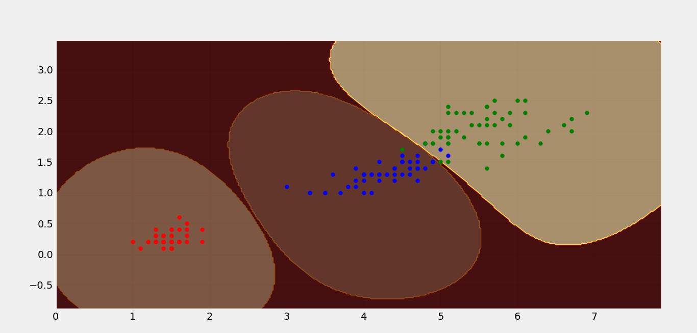

上图显示了 IRIS 数据集的三类分类。

1. From sklearn, we imported the SVM library.
2. We created 3 non-linear SVM’s (RBF kernel based).
3. Each SVM was fed with 1 class kept positive and other 2 as negative. Say, SVM1 had labels corresponding to class 1 only else all were made 0. Same for SVM2 and SVM3 respectively.
4. Plot the contour plot of each SVM.
5. Plot the data points.

下面是相同的Python实现。

import numpy as np 
import pandas as pd 
import matplotlib.pyplot as plt 
from matplotlib import style
from sklearn.svm import SVC 
  
style.use('fivethirtyeight')
  
# create mesh grids
def make_meshgrid(x, y, h =.02):
    x_min, x_max = x.min() - 1, x.max() + 1
    y_min, y_max = y.min() - 1, y.max() + 1
    xx, yy = np.meshgrid(np.arange(x_min, x_max, h), np.arange(y_min, y_max, h))
    return xx, yy
  
# plot the contours
def plot_contours(ax, clf, xx, yy, **params):
    Z = clf.predict(np.c_[xx.ravel(), yy.ravel()])
    Z = Z.reshape(xx.shape)
    out = ax.contourf(xx, yy, Z, **params)
    return out
  
color = ['r', 'b', 'g', 'k']
  
iris = pd.read_csv("iris-data.txt").values
  
  
features = iris[0:150, 2:4]
level1 = np.zeros(150)
level2 = np.zeros(150)
level3 = np.zeros(150)
  
# level1 contains 1 for class1 and 0 for all others.
# level2 contains 1 for class2 and 0 for all others.
# level3 contains 1 for class3 and 0 for all others.
for i in range(150):
    if i>= 0 and i<50:
        level1[i] = 1
    elif i>= 50 and i<100:
        level2[i] = 1
    elif i>= 100 and i<150:
        level3[i]= 1
  
# create 3 svm with rbf kernels
svm1 = SVC(kernel ='rbf')
svm2 = SVC(kernel ='rbf')
svm3 = SVC(kernel ='rbf')
  
# fit each svm's
svm1.fit(features, level1)
svm2.fit(features, level2)
svm3.fit(features, level3)
  
fig, ax = plt.subplots()
X0, X1 = iris[:, 2], iris[:, 3]
xx, yy = make_meshgrid(X0, X1)
  
# plot the contours
plot_contours(ax, svm1, xx, yy, cmap = plt.get_cmap('hot'), alpha = 0.8)
plot_contours(ax, svm2, xx, yy, cmap = plt.get_cmap('hot'), alpha = 0.3)
plot_contours(ax, svm3, xx, yy, cmap = plt.get_cmap('hot'), alpha = 0.5)
  
color = ['r', 'b', 'g', 'k']
  
for i in range(len(iris)):
    plt.scatter(iris[i][2], iris[i][3], s = 30, c = color[int(iris[i][4])])
plt.show()