Scikit学习-支持向量机

📌 相关文章

📜 Scikit学习-支持向量机

📅 最后修改于: 2020-12-10 05:51:36 🧑 作者: Mango

本章介绍了一种称为支持向量机(SVM)的机器学习方法。

介绍

支持向量机(SVM)是强大而灵活的监督型机器学习方法，用于分类，回归和离群值检测。 SVM在高维空间中非常有效，通常用于分类问题。 SVM受欢迎且具有存储效率，因为它们在决策函数使用训练点的子集。

SVM的主要目标是将数据集分为几类，以找到最大的边际超平面(MMH) ，可以在以下两个步骤中完成-

支持向量机将首先以迭代方式生成超平面，从而以最佳方式分隔类。
之后，它将选择正确隔离类的超平面。

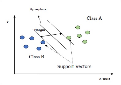
SVM中的一些重要概念如下-

支持向量-它们可以定义为最接近超平面的数据点。支持向量有助于确定分隔线。
超平面-划分具有不同类别的对象集的决策平面或空间。
裕度-不同类别的壁橱数据点上的两条线之间的间隙称为裕度。

下图将为您提供有关这些SVM概念的见解-

边缘超平面

Scikit-learn中的SVM支持稀疏和密集样本矢量作为输入。

支持向量机的分类

Scikit-learn提供三个类，即SVC，NuSVC和LinearSVC ，它们可以执行多类分类。

SVC

这是C支持向量分类，其实现基于libsvm 。 scikit-learn使用的模块是sklearn.svm.SVC 。此类根据一对一方案处理多类支持。

参量

followings表包含sklearn.svm.SVC类使用的参数-

Sr.No	Parameter & Description
1	C − float, optional, default = 1.0 It is the penalty parameter of the error term.
2	kernel − string, optional, default = ‘rbf’ This parameter specifies the type of kernel to be used in the algorithm. we can choose any one among, ‘linear’, ‘poly’, ‘rbf’, ‘sigmoid’, ‘precomputed’. The default value of kernel would be ‘rbf’.
3	degree − int, optional, default = 3 It represents the degree of the ‘poly’ kernel function and will be ignored by all other kernels.
4	gamma − {‘scale’, ‘auto’} or float, It is the kernel coefficient for kernels ‘rbf’, ‘poly’ and ‘sigmoid’.
5	optinal default − = ‘scale’ If you choose default i.e. gamma = ‘scale’ then the value of gamma to be used by SVC is 1/(𝑛_𝑓𝑒𝑎𝑡𝑢𝑟𝑒𝑠∗𝑋.𝑣𝑎𝑟()). On the other hand, if gamma= ‘auto’, it uses 1/𝑛_𝑓𝑒𝑎𝑡𝑢𝑟𝑒𝑠.
6	coef0 − float, optional, Default=0.0 An independent term in kernel function which is only significant in ‘poly’ and ‘sigmoid’.
7	tol − float, optional, default = 1.e-3 This parameter represents the stopping criterion for iterations.
8	shrinking − Boolean, optional, default = True This parameter represents that whether we want to use shrinking heuristic or not.
9	verbose − Boolean, default: false It enables or disable verbose output. Its default value is false.
10	probability − boolean, optional, default = true This parameter enables or disables probability estimates. The default value is false, but it must be enabled before we call fit.
11	max_iter − int, optional, default = -1 As name suggest, it represents the maximum number of iterations within the solver. Value -1 means there is no limit on the number of iterations.
12	cache_size − float, optional This parameter will specify the size of the kernel cache. The value will be in MB(MegaBytes).
13	random_state − int, RandomState instance or None, optional, default = none This parameter represents the seed of the pseudo random number generated which is used while shuffling the data. Followings are the options − int − In this case, random_state is the seed used by random number generator. RandomState instance − In this case, random_state is the random number generator. None − In this case, the random number generator is the RandonState instance used by np.random.
14	class_weight − {dict, ‘balanced’}, optional This parameter will set the parameter C of class j to 𝑐𝑙𝑎𝑠𝑠_𝑤𝑒𝑖𝑔ℎ𝑡[𝑗]∗𝐶 for SVC. If we use the default option, it means all the classes are supposed to have weight one. On the other hand, if you choose *class_weight:balanced*, it will use the values of y to automatically adjust weights.
15	decision_function_shape − ovo’, ‘ovr’, default = ‘ovr’ This parameter will decide whether the algorithm will return ‘ovr’ (one-vs-rest) decision function of shape as all other classifiers, or the original ovo(one-vs-one) decision function of libsvm.
16	break_ties − boolean, optional, default = false True − The predict will break ties according to the confidence values of decision_function False − The predict will return the first class among the tied classes.

属性

followings表包含sklearn.svm.SVC类使用的属性-

Sr.No	Attributes & Description
1	support_ − array-like, shape = [n_SV] It returns the indices of support vectors.
2	support_vectors_ − array-like, shape = [n_SV, n_features] It returns the support vectors.
3	n_support_ − array-like, dtype=int32, shape = [n_class] It represents the number of support vectors for each class.
4	dual_coef_ − array, shape = [n_class-1,n_SV] These are the coefficient of the support vectors in the decision function.
5	coef_ − array, shape = [n_class * (n_class-1)/2, n_features] This attribute, only available in case of linear kernel, provides the weight assigned to the features.
6	intercept_ − array, shape = [n_class * (n_class-1)/2] It represents the independent term (constant) in decision function.
7	fit_status_ − int The output would be 0 if it is correctly fitted. The output would be 1 if it is incorrectly fitted.
8	classes_ − array of shape = [n_classes] It gives the labels of the classes.

实施实例

像其他分类器一样，SVC还必须配备以下两个数组-

存放训练样本的数组X。它的大小为[n_samples，n_features]。
保存目标值的数组Y ，即训练样本的类别标签。它的大小为[n_samples]。

以下Python脚本使用sklearn.svm.SVC类-

import numpy as np
X = np.array([[-1, -1], [-2, -1], [1, 1], [2, 1]])
y = np.array([1, 1, 2, 2])
from sklearn.svm import SVC
SVCClf = SVC(kernel = 'linear',gamma = 'scale', shrinking = False,)
SVCClf.fit(X, y)

输出

SVC(C = 1.0, cache_size = 200, class_weight = None, coef0 = 0.0,
   decision_function_shape = 'ovr', degree = 3, gamma = 'scale', kernel = 'linear',
   max_iter = -1, probability = False, random_state = None, shrinking = False,
   tol = 0.001, verbose = False)

例

现在，一旦拟合，我们就可以在以下Python脚本的帮助下获得权重向量-

SVCClf.coef_

输出

array([[0.5, 0.5]])

例

类似地，我们可以获取其他属性的值，如下所示：

SVCClf.predict([[-0.5,-0.8]])

输出

array([1])

例

SVCClf.n_support_

输出

array([1, 1])

例

SVCClf.support_vectors_

输出

array(
   [
      [-1., -1.],
      [ 1., 1.]
   ]
)

例

SVCClf.support_

输出

array([0, 2])

例

SVCClf.intercept_

输出

array([-0.])

例

SVCClf.fit_status_

输出

NuSVC

NuSVC是Nu支持向量分类。它是scikit-learn提供的另一个类，可以执行多类分类。就像SVC一样，但是NuSVC接受略有不同的参数集。与SVC不同的参数如下-

nu-浮动，可选，默认= 0.5

它代表训练误差分数的上限和支持向量分数的下限。其值应在(o，1]的间隔内。

其余参数和属性与SVC相同。

实施实例

我们也可以使用sklearn.svm.NuSVC类实现相同的示例。

import numpy as np
X = np.array([[-1, -1], [-2, -1], [1, 1], [2, 1]])
y = np.array([1, 1, 2, 2])
from sklearn.svm import NuSVC
NuSVCClf = NuSVC(kernel = 'linear',gamma = 'scale', shrinking = False,)
NuSVCClf.fit(X, y)

输出

NuSVC(cache_size = 200, class_weight = None, coef0 = 0.0,
   decision_function_shape = 'ovr', degree = 3, gamma = 'scale', kernel = 'linear',
   max_iter = -1, nu = 0.5, probability = False, random_state = None,
   shrinking = False, tol = 0.001, verbose = False)

我们可以像SVC一样获得其余属性的输出。

线性SVC

这是线性支持向量分类。它类似于具有内核=“线性”的SVC。它们之间的区别在于LinearSVC是根据liblinear实现的，而SVC是在libsvm中实现的。这就是LinearSVC在罚分和损失函数选择方面具有更大灵活性的原因。它还可以更好地扩展到大量样本。

如果我们谈论它的参数和属性，那么它就不支持“内核”，因为它被认为是线性的，并且还缺少一些属性，例如support_，support_vectors_，n_support_，fit_status_和dual_coef_ 。

但是，它支持惩罚和损失参数，如下所示：

惩罚-字符串，L1或L2(默认=’L2’)

此参数用于指定惩罚(正则化)中使用的标准(L1或L2)。
loss-字符串，铰链，squared_hinge(默认= squared_hinge)

它表示损耗函数，其中“铰链”是标准SVM损耗，“ squared_hinge”是铰链损耗的平方。

实施实例

以下Python脚本使用sklearn.svm.LinearSVC类-

from sklearn.svm import LinearSVC
from sklearn.datasets import make_classification
X, y = make_classification(n_features = 4, random_state = 0)
LSVCClf = LinearSVC(dual = False, random_state = 0, penalty = 'l1',tol = 1e-5)
LSVCClf.fit(X, y)

输出

LinearSVC(C = 1.0, class_weight = None, dual = False, fit_intercept = True,
   intercept_scaling = 1, loss = 'squared_hinge', max_iter = 1000,
   multi_class = 'ovr', penalty = 'l1', random_state = 0, tol = 1e-05, verbose = 0)

例

现在，一旦拟合，模型可以预测新值，如下所示：

LSVCClf.predict([[0,0,0,0]])

输出

[1]

例

对于上面的示例，我们可以借助以下Python脚本获取权重向量-

LSVCClf.coef_

输出

[[0. 0. 0.91214955 0.22630686]]

例

同样，我们可以在以下Python脚本的帮助下获取拦截的值-

LSVCClf.intercept_

输出

[0.26860518]

支持向量机回归

如前所述，SVM用于分类和回归问题。 Scikit-learn的支持向量分类(SVC)方法也可以扩展为解决回归问题。该扩展方法称为支持向量回归(SVR)。

SVM和SVR之间的基本相似之处

SVC创建的模型仅取决于训练数据的子集。为什么?因为构建模型的成本函数并不关心位于边距之外的训练数据点。

而SVR(支持向量回归)产生的模型也仅取决于训练数据的子集。为什么?因为用于构建模型的成本函数忽略任何接近模型预测的训练数据点。

Scikit-learn提供了三个类，即SVR，NuSVR和LinearSVR，作为SVR的三种不同实现。

SVR

这是Epsilon支持的向量回归，其实现基于libsvm 。与SVC相反，模型中有两个自由参数，即‘C’和‘epsilon’ 。

epsilon-浮动，可选，默认= 0.1

它代表epsilon-SVR模型中的epsilon，并指定在epsilon-tube中训练损失函数与从实际值算起的距离epsilon中预测的点无关的惩罚。

其余的参数和属性与我们在SVC中使用的相似。

实施实例

以下Python脚本使用sklearn.svm.SVR类-

from sklearn import svm
X = [[1, 1], [2, 2]]
y = [1, 2]
SVRReg = svm.SVR(kernel = ’linear’, gamma = ’auto’)
SVRReg.fit(X, y)

输出

SVR(C = 1.0, cache_size = 200, coef0 = 0.0, degree = 3, epsilon = 0.1, gamma = 'auto',
   kernel = 'linear', max_iter = -1, shrinking = True, tol = 0.001, verbose = False)

例

现在，一旦拟合，我们就可以在以下Python脚本的帮助下获得权重向量-

SVRReg.coef_

输出

array([[0.4, 0.4]])

例

类似地，我们可以获取其他属性的值，如下所示：

SVRReg.predict([[1,1]])

输出

array([1.1])

同样，我们也可以获取其他属性的值。

NuSVR

NuSVR是Nu支持向量回归。就像NuSVC一样，但是NuSVR使用参数nu来控制支持向量的数量。而且，与NuSVC的nu替换了C参数不同，此处它替换了epsilon 。

实施实例

以下Python脚本使用sklearn.svm.SVR类-

from sklearn.svm import NuSVR
import numpy as np
n_samples, n_features = 20, 15
np.random.seed(0)
y = np.random.randn(n_samples)
X = np.random.randn(n_samples, n_features)
NuSVRReg = NuSVR(kernel = 'linear', gamma = 'auto',C = 1.0, nu = 0.1)^M
NuSVRReg.fit(X, y)

输出

NuSVR(C = 1.0, cache_size = 200, coef0 = 0.0, degree = 3, gamma = 'auto',
   kernel = 'linear', max_iter = -1, nu = 0.1, shrinking = True, tol = 0.001,
   verbose = False)

例

现在，一旦拟合，我们就可以在以下Python脚本的帮助下获得权重向量-

NuSVRReg.coef_

输出

array(
   [
      [-0.14904483, 0.04596145, 0.22605216, -0.08125403, 0.06564533,
      0.01104285, 0.04068767, 0.2918337 , -0.13473211, 0.36006765,
      -0.2185713 , -0.31836476, -0.03048429, 0.16102126, -0.29317051]
   ]
)

同样，我们也可以获取其他属性的值。

线性SVR

它是线性支持向量回归。它类似于具有内核=“线性”的SVR。它们之间的区别是，在LinearSVR的liblinear方面实施，而SVC在LIBSVM实现。这就是LinearSVR在罚分和损失函数选择方面更具灵活性的原因。它还可以更好地扩展到大量样本。

但是，它支持以下“损失”参数-

loss-字符串，可选，默认=’epsilon_insensitive’

它表示损失函数，其中epsilon_insensitive损失是L1损失，平方的epsilon_insensitive损失是L2损失。

实施实例

以下Python脚本使用sklearn.svm.LinearSVR类-

from sklearn.svm import LinearSVR
from sklearn.datasets import make_regression
X, y = make_regression(n_features = 4, random_state = 0)
LSVRReg = LinearSVR(dual = False, random_state = 0,
loss = 'squared_epsilon_insensitive',tol = 1e-5)
LSVRReg.fit(X, y)

输出

LinearSVR(
   C=1.0, dual=False, epsilon=0.0, fit_intercept=True,
   intercept_scaling=1.0, loss='squared_epsilon_insensitive',
   max_iter=1000, random_state=0, tol=1e-05, verbose=0
)

例

现在，一旦拟合，模型可以预测新值，如下所示：

LSRReg.predict([[0,0,0,0]])

输出

array([-0.01041416])

例

对于上面的示例，我们可以借助以下Python脚本获取权重向量-

LSRReg.coef_

输出

array([20.47354746, 34.08619401, 67.23189022, 87.47017787])

例

同样，我们可以在以下Python脚本的帮助下获取拦截的值-

LSRReg.intercept_

输出

array([-0.01041416])