毫升 |均值漂移聚类

与无监督学习相比， Meanshift属于聚类算法的类别，无监督学习通过将点移向模式迭代地将数据点分配给集群（模式是该区域中数据点的最高密度，在 Meanshift 的上下文中） .因此，它也被称为寻模算法。 Mean-shift算法在图像处理和计算机视觉领域都有应用。

Given a set of data points, the algorithm iteratively assigns each data point towards the closest cluster centroid and direction to the closest cluster centroid is determined by where most of the points nearby are at. So each iteration each data point will move closer to where the most points are at, which is or will lead to the cluster center. When the algorithm stops, each point is assigned to a cluster.

编程需要懂一点英语

与流行的 K-Means 聚类算法不同，mean-shift 不需要提前指定聚类的数量。聚类的数量由算法相对于数据确定。

注意： Mean Shift 的缺点是计算量大 O(n²)。

核密度估计——

应用均值偏移聚类算法的第一步是以数学方式表示您的数据，这意味着将您的数据表示为点，如下面的集合。

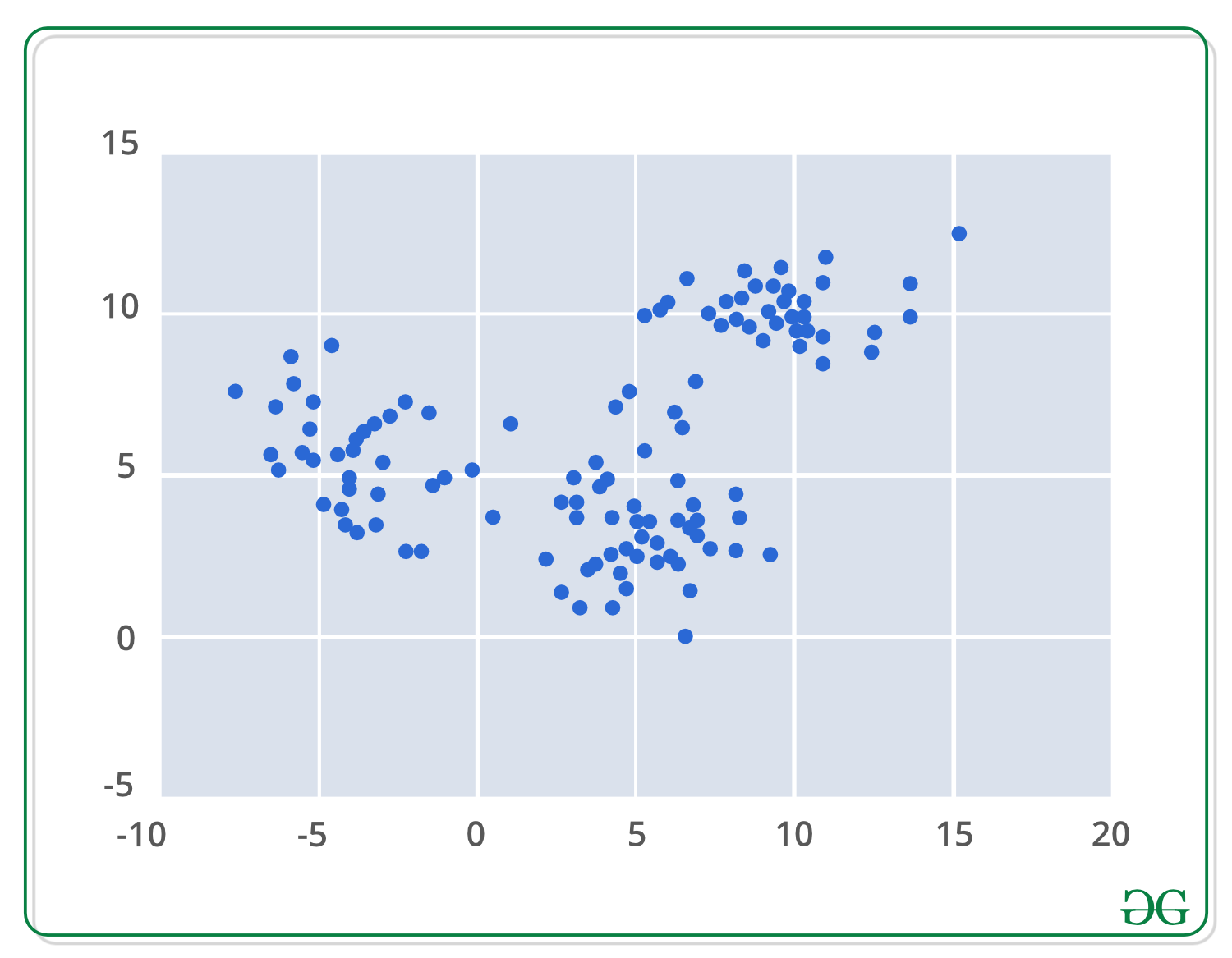
Mean-shift 基于核密度估计的概念，简称 KDE。想象一下，上述数据是从概率分布中采样的。 KDE 是一种估计基础分布的方法，也称为一组数据的概率密度函数。

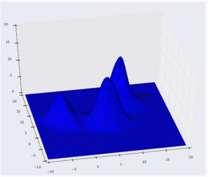
它通过在数据集中的每个点上放置一个内核来工作。内核是通常用于卷积的加权函数的一个花哨的数学词。有许多不同类型的内核，但最流行的一种是高斯内核。将所有单独的内核相加会生成一个概率表面示例密度函数。根据使用的内核带宽参数，最终的密度函数会有所不同。

下面是我们使用内核带宽为 2 的高斯内核的上述点的 KDE 表面。

曲面图：

等高线图：

以下是Python实现：

import numpy as np
import pandas as pd
from sklearn.cluster import MeanShift
from sklearn.datasets.samples_generator import make_blobs
from matplotlib import pyplot as plt
from mpl_toolkits.mplot3d import Axes3D
   
# We will be using the make_blobs method
# in order to generate our own data.
  
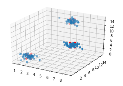
clusters = [[2, 2, 2], [7, 7, 7], [5, 13, 13]]
  
X, _ = make_blobs(n_samples = 150, centers = clusters,
                                   cluster_std = 0.60)
   
# After training the model, We store the
# coordinates for the cluster centers
ms = MeanShift()
ms.fit(X)
cluster_centers = ms.cluster_centers_
   
# Finally We plot the data points
# and centroids in a 3D graph.
fig = plt.figure()
  
ax = fig.add_subplot(111, projection ='3d')
  
ax.scatter(X[:, 0], X[:, 1], X[:, 2], marker ='o')
  
ax.scatter(cluster_centers[:, 0], cluster_centers[:, 1],
           cluster_centers[:, 2], marker ='x', color ='red',
           s = 300, linewidth = 5, zorder = 10)
  
plt.show()

在此处尝试代码

输出：

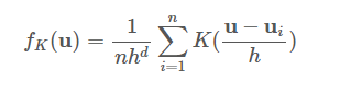
为了说明，假设我们有一个 d 维空间中点的数据集 {ui}，从一些更大的总体中采样，并且我们选择了一个具有带宽参数 h 的内核 K。这些数据和核函数一起返回完整人口密度函数的以下核密度估计量。

这里的核函数需要满足以下两个条件：

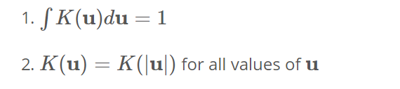
-> The first requirement is needed to ensure that our estimate is normalized.
-> The second is associated with the symmetry of our space.

编程需要懂一点英语

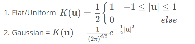
满足这些条件的两个流行的内核函数由-

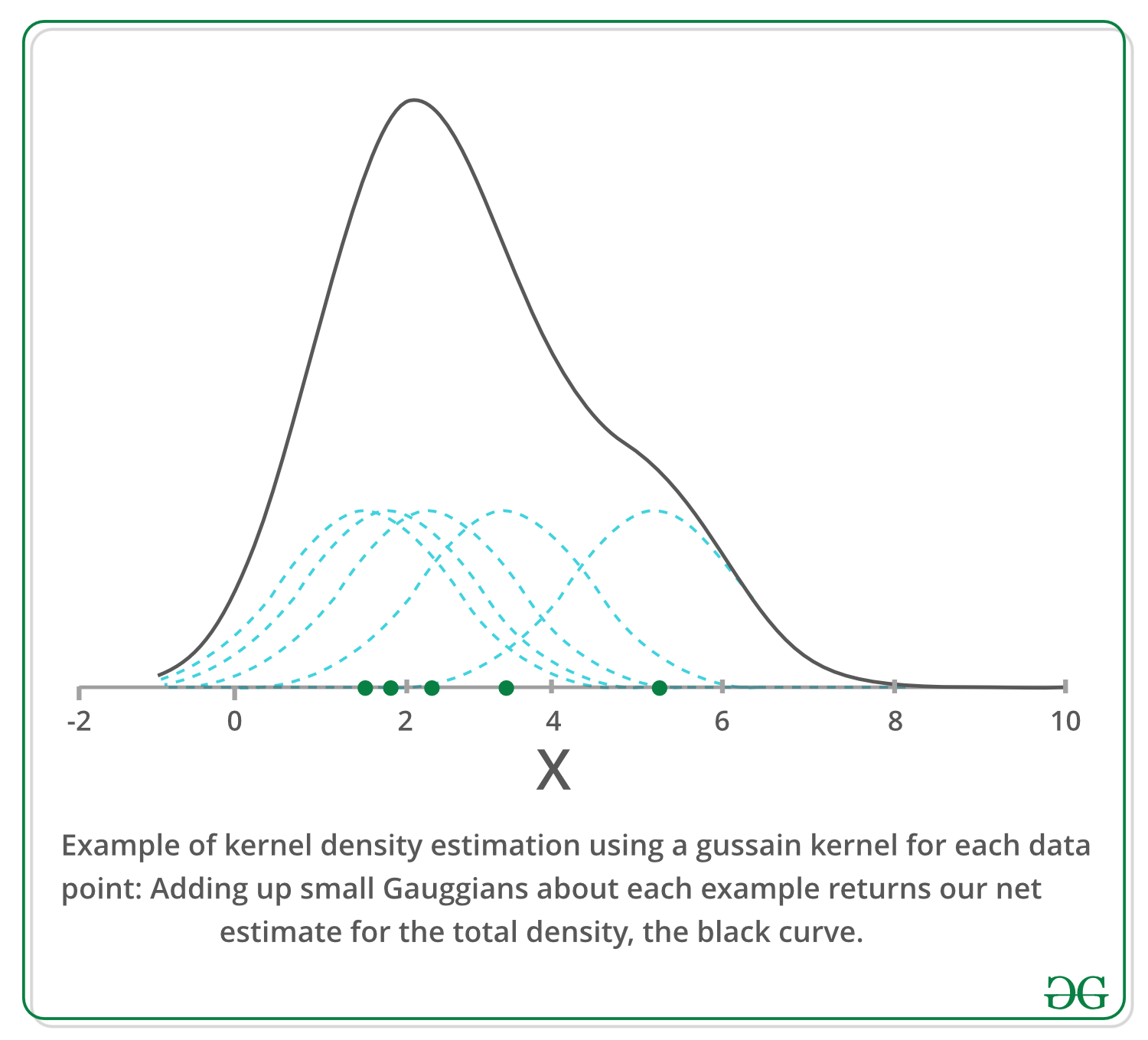
下面我们使用高斯核在一维中绘制一个示例，以估计一些人口沿 x 轴的密度。我们可以看到，每个样本点都为我们的估计增加了一个小高斯，以它为中心，上面的方程可能看起来有点吓人，但这里的图形应该清楚地说明这个概念非常简单。

迭代模式搜索 –

1. Initialize random seed and window W.
2. Calculate the center of gravity (mean) of W.    
3. Shift the search window to the mean.    
4. Repeat Step 2 until convergence.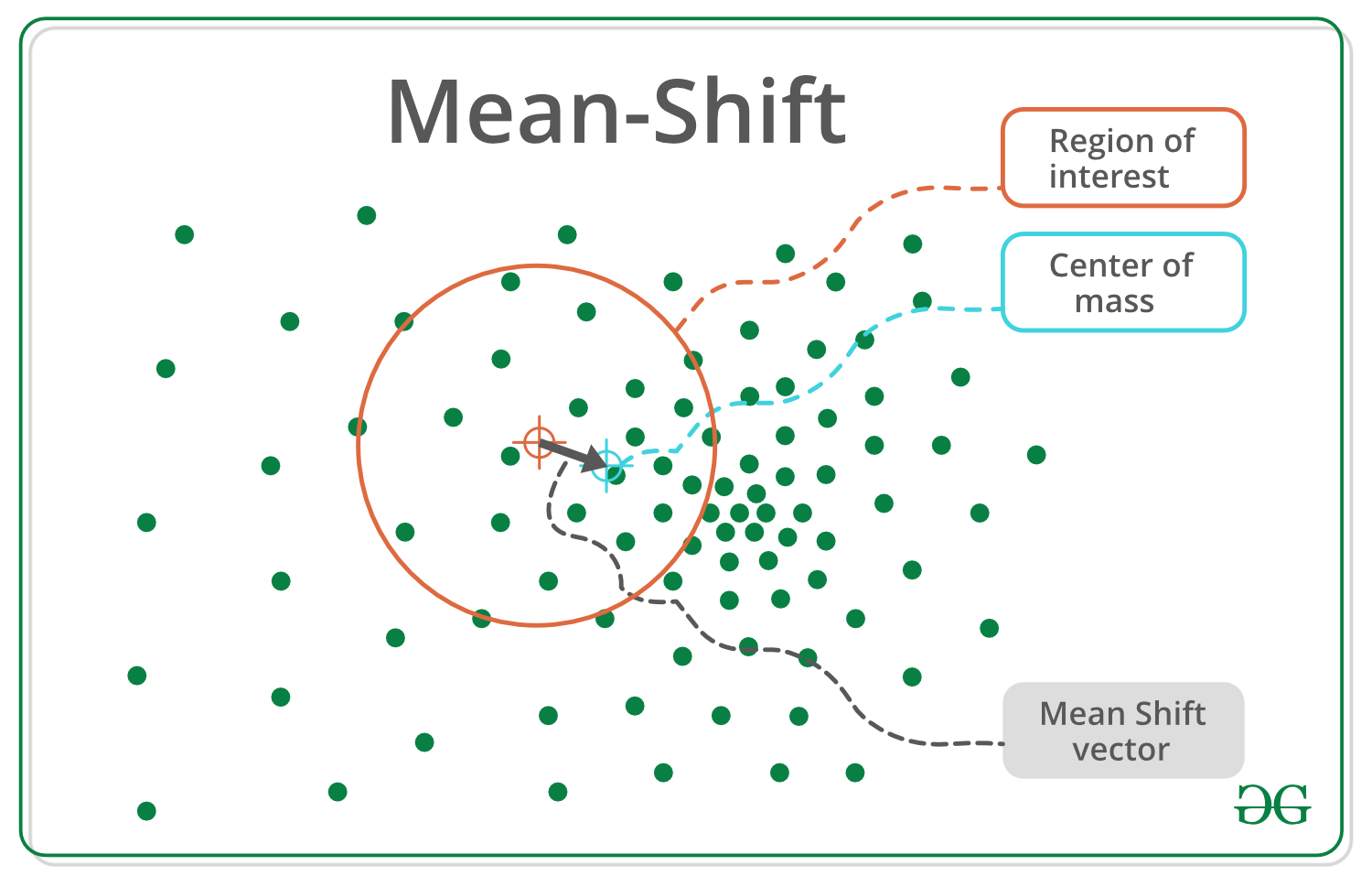

一般算法大纲 –

for p in copied_points:
    while not at_kde_peak:
        p = shift(p, original_points)

Shift函数如下所示 -

def shift(p, original_points):
    shift_x = float(0)
    shift_y = float(0)
    scale_factor = float(0)
  
    for p_temp in original_points:
        # numerator
        dist = euclidean_dist(p, p_temp)
        weight = kernel(dist, kernel_bandwidth)
        shift_x += p_temp[0] * weight
        shift_y += p_temp[1] * weight
        # denominator
        scale_factor += weight
  
    shift_x = shift_x / scale_factor
    shift_y = shift_y / scale_factor
    return [shift_x, shift_y]

优点：

查找可变数量的模式
对异常值鲁棒
通用的、独立于应用程序的工具
无模型，在数据集群上不假设任何先前的形状，如球形、椭圆形等
只有一个参数（窗口大小 h），其中 h 具有物理意义（与 k-means 不同）

缺点：

输出取决于窗口大小
窗口大小（带宽）selecHon 不是微不足道的
计算上（相对）昂贵（大约 2 秒/图像）
不能很好地与特征空间的维度一起缩放。