使用 Matplotlib 在Python中绘制直方图

直方图基本上用于表示以某些组的形式提供的数据。它是数字数据分布的图形表示的准确方法。它是一种条形图，其中 X 轴表示 bin 范围，而 Y 轴给出信息关于频率。

创建直方图

要创建直方图，第一步是创建范围的 bin，然后将值的整个范围分布到一系列区间中，并对落入每个区间的值进行计数。Bins 被清楚地标识为连续的、非变量的重叠区间。matplotlib.pyplot.hist()函数用于计算和创建 x 的直方图。

下表显示了 matplotlib.pyplot.hist()函数接受的参数：

Attribute	parameter
x	array or sequence of array
bins	optional parameter contains integer or sequence or strings
density	optional parameter contains boolean values
range	optional parameter represents upper and lower range of bins
histtype	optional parameter used to create type of histogram [bar, barstacked, step, stepfilled], default is “bar”
align	optional parameter controls the plotting of histogram [left, right, mid]
weights	optional parameter contains array of weights having same dimensions as x
bottom	location of the basline of each bin
rwidth	optional parameter which is relative width of the bars with respect to bin width
color	optional parameter used to set color or sequence of color specs
label	optional parameter string or sequence of string to match with multiple datasets
log	optional parameter used to set histogram axis on log scale

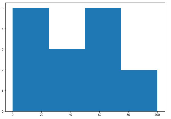
让我们创建一些随机值的基本直方图。下面的代码创建了一些随机值的简单直方图：

Python3

from matplotlib import pyplot as plt
import numpy as np
 
 
# Creating dataset
a = np.array([22, 87, 5, 43, 56,
              73, 55, 54, 11,
              20, 51, 5, 79, 31,
              27])
 
# Creating histogram
fig, ax = plt.subplots(figsize =(10, 7))
ax.hist(a, bins = [0, 25, 50, 75, 100])
 
# Show plot
plt.show()

输出 ：

直方图自定义

Matplotlib 提供了一系列不同的方法来自定义直方图。
matplotlib.pyplot.hist()函数本身提供了许多属性，借助这些属性我们可以修改直方图。 hist()函数提供了一个补丁对象，它可以访问创建对象的属性，使用它我们可以修改绘图按照我们的意愿。

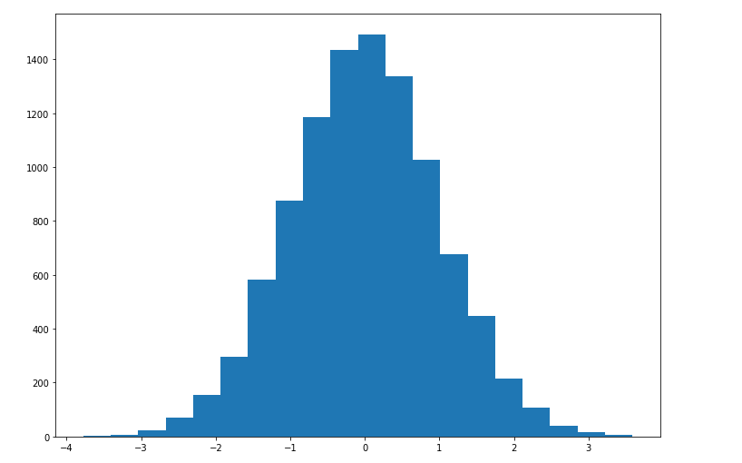
示例 1：

Python3

import matplotlib.pyplot as plt
import numpy as np
from matplotlib import colors
from matplotlib.ticker import PercentFormatter
 
# Creating dataset
np.random.seed(23685752)
N_points = 10000
n_bins = 20
 
# Creating distribution
x = np.random.randn(N_points)
y = .8 ** x + np.random.randn(10000) + 25
 
# Creating histogram
fig, axs = plt.subplots(1, 1,
                        figsize =(10, 7),
                        tight_layout = True)
 
axs.hist(x, bins = n_bins)
 
# Show plot
plt.show()

输出 ：

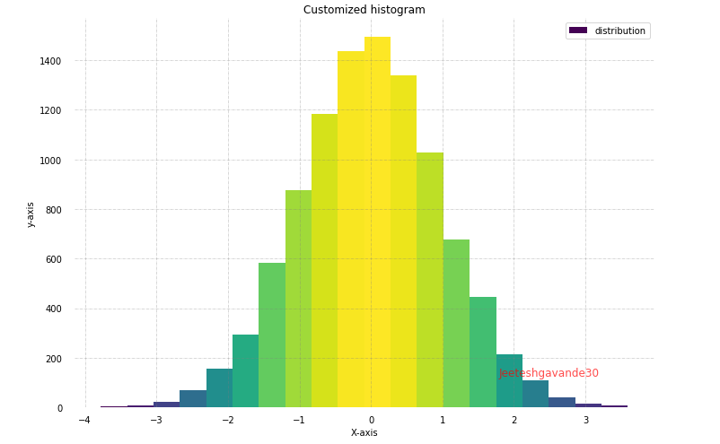
示例 2：下面的代码修改了上面的直方图以获得更好的视图和准确的读数。

Python3

import matplotlib.pyplot as plt
import numpy as np
from matplotlib import colors
from matplotlib.ticker import PercentFormatter
 
 
# Creating dataset
np.random.seed(23685752)
N_points = 10000
n_bins = 20
 
# Creating distribution
x = np.random.randn(N_points)
y = .8 ** x + np.random.randn(10000) + 25
legend = ['distribution']
 
# Creating histogram
fig, axs = plt.subplots(1, 1,
                        figsize =(10, 7),
                        tight_layout = True)
 
 
# Remove axes splines
for s in ['top', 'bottom', 'left', 'right']:
    axs.spines[s].set_visible(False)
 
# Remove x, y ticks
axs.xaxis.set_ticks_position('none')
axs.yaxis.set_ticks_position('none')
   
# Add padding between axes and labels
axs.xaxis.set_tick_params(pad = 5)
axs.yaxis.set_tick_params(pad = 10)
 
# Add x, y gridlines
axs.grid(b = True, color ='grey',
        linestyle ='-.', linewidth = 0.5,
        alpha = 0.6)
 
# Add Text watermark
fig.text(0.9, 0.15, 'Jeeteshgavande30',
         fontsize = 12,
         color ='red',
         ha ='right',
         va ='bottom',
         alpha = 0.7)
 
# Creating histogram
N, bins, patches = axs.hist(x, bins = n_bins)
 
# Setting color
fracs = ((N**(1 / 5)) / N.max())
norm = colors.Normalize(fracs.min(), fracs.max())
 
for thisfrac, thispatch in zip(fracs, patches):
    color = plt.cm.viridis(norm(thisfrac))
    thispatch.set_facecolor(color)
 
# Adding extra features   
plt.xlabel("X-axis")
plt.ylabel("y-axis")
plt.legend(legend)
plt.title('Customized histogram')
 
# Show plot
plt.show()

输出 ：