使用 Sklearn 实现凝聚聚类

先决条件：凝聚聚类
凝聚聚类是最常见的层次聚类技术之一。
数据集——信用卡数据集。

假设：聚类技术假设每个数据点与其他数据点足够相似，因此可以假设开始时的数据被聚类在 1 个集群中。

第 1 步：导入所需的库

import pandas as pd
import numpy as np
import matplotlib.pyplot as plt
from sklearn.decomposition import PCA
from sklearn.cluster import AgglomerativeClustering
from sklearn.preprocessing import StandardScaler, normalize
from sklearn.metrics import silhouette_score
import scipy.cluster.hierarchy as shc

第 2 步：加载和清理数据

# Changing the working location to the location of the file
cd C:\Users\Dev\Desktop\Kaggle\Credit_Card
  
X = pd.read_csv('CC_GENERAL.csv')
  
# Dropping the CUST_ID column from the data
X = X.drop('CUST_ID', axis = 1)
  
# Handling the missing values
X.fillna(method ='ffill', inplace = True)

第 3 步：预处理数据

# Scaling the data so that all the features become comparable
scaler = StandardScaler()
X_scaled = scaler.fit_transform(X)
  
# Normalizing the data so that the data approximately 
# follows a Gaussian distribution
X_normalized = normalize(X_scaled)
  
# Converting the numpy array into a pandas DataFrame
X_normalized = pd.DataFrame(X_normalized)

第 4 步：降低数据的维度

pca = PCA(n_components = 2)
X_principal = pca.fit_transform(X_normalized)
X_principal = pd.DataFrame(X_principal)
X_principal.columns = ['P1', 'P2']

树状图用于将给定的集群划分为许多不同的集群。

第 5 步：可视化树状图的工作

plt.figure(figsize =(8, 8))
plt.title('Visualising the data')
Dendrogram = shc.dendrogram((shc.linkage(X_principal, method ='ward')))

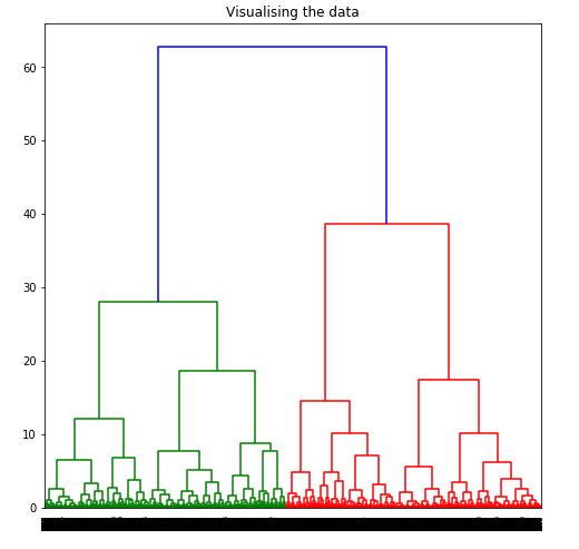
要通过可视化数据来确定最佳聚类数，将所有水平线想象为完全水平，然后在计算任意两条水平线之间的最大距离后，在计算出的最大距离处绘制一条水平线。

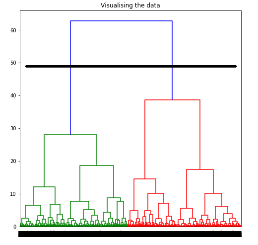
上图显示，对于给定数据，最佳聚类数应为 2。

第 6 步：针对不同的 k 值构建和可视化不同的聚类模型

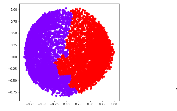
a) k = 2

ac2 = AgglomerativeClustering(n_clusters = 2)
  
# Visualizing the clustering
plt.figure(figsize =(6, 6))
plt.scatter(X_principal['P1'], X_principal['P2'], 
           c = ac2.fit_predict(X_principal), cmap ='rainbow')
plt.show()

b) k = 3

ac3 = AgglomerativeClustering(n_clusters = 3)
  
plt.figure(figsize =(6, 6))
plt.scatter(X_principal['P1'], X_principal['P2'],
           c = ac3.fit_predict(X_principal), cmap ='rainbow')
plt.show()

c) k = 4

ac4 = AgglomerativeClustering(n_clusters = 4)
  
plt.figure(figsize =(6, 6))
plt.scatter(X_principal['P1'], X_principal['P2'],
            c = ac4.fit_predict(X_principal), cmap ='rainbow')
plt.show()

d) k = 5

ac5 = AgglomerativeClustering(n_clusters = 5)
  
plt.figure(figsize =(6, 6))
plt.scatter(X_principal['P1'], X_principal['P2'],
            c = ac5.fit_predict(X_principal), cmap ='rainbow')
plt.show()

e) k = 6

ac6 = AgglomerativeClustering(n_clusters = 6)
  
plt.figure(figsize =(6, 6))
plt.scatter(X_principal['P1'], X_principal['P2'],
            c = ac6.fit_predict(X_principal), cmap ='rainbow')
plt.show()

我们现在使用数学技术确定最佳聚类数。在这里，我们将为此目的使用剪影分数。

第 7 步：评估不同的模型并可视化结果。

k = [2, 3, 4, 5, 6]
  
# Appending the silhouette scores of the different models to the list
silhouette_scores = []
silhouette_scores.append(
        silhouette_score(X_principal, ac2.fit_predict(X_principal)))
silhouette_scores.append(
        silhouette_score(X_principal, ac3.fit_predict(X_principal)))
silhouette_scores.append(
        silhouette_score(X_principal, ac4.fit_predict(X_principal)))
silhouette_scores.append(
        silhouette_score(X_principal, ac5.fit_predict(X_principal)))
silhouette_scores.append(
        silhouette_score(X_principal, ac6.fit_predict(X_principal)))
  
# Plotting a bar graph to compare the results
plt.bar(k, silhouette_scores)
plt.xlabel('Number of clusters', fontsize = 20)
plt.ylabel('S(i)', fontsize = 20)
plt.show()

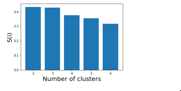
因此，在轮廓分数的帮助下，可以得出结论，给定数据和聚类技术的最佳聚类数为 2。