R 编程中的探索性数据分析
探索性数据分析或 EDA是一种统计方法或技术,用于分析数据集,以便通过使用一些视觉辅助工具概括其重要和主要特征。 EDA 方法可用于收集有关以下数据方面的知识:
- 数据的主要特征或特征。
- 变量及其关系。
- 找出可以在我们的问题中使用的重要变量。
EDA 是一种迭代方法,包括:
- 产生有关我们数据的问题
- 通过对我们的数据进行可视化、转换和建模来寻找答案。
- 使用我们学到的经验来改进我们的问题集或生成一组新问题。
R中的探索性数据分析
在 R 语言中,我们将在两大类下执行 EDA:
- 描述性统计,包括平均值、中位数、众数、四分位间距等。
- 图形方法,包括直方图、密度估计、箱线图等。
在我们开始使用 EDA 之前,我们必须正确执行数据检查。在我们的分析中,我们将使用 R 中的soilDB包中的loafercreek 。我们将检查我们的数据以找出所有的拼写错误和明显的错误。进一步的 EDA 可用于确定和识别异常值并执行所需的统计分析。为了执行 EDA,我们必须安装并加载以下包:
- “aqp”包
- “ggplot2”包
- “土壤数据库”包
我们可以使用install.packages()命令从 R 控制台安装这些包,并使用library()命令将它们加载到我们的 R 脚本中。我们现在将看到如何检查我们的数据并删除拼写错误和明显的错误。
R中EDA的数据检查
为了确保我们处理正确的信息,我们需要在转换过程的每个阶段清楚地查看您的数据。数据检查是在翻译之前、期间或之后查看数据以进行验证和调试的行为。现在让我们看看如何检查和删除数据中的错误和拼写错误。
例子:
R
# Data Inspection in EDA
# loading the required packages
library(aqp)
library(soilDB)

# Load from the the loakercreek dataset
data("loafercreek")

# Construct generalized horizon designations
n < - c("A", "BAt", "Bt1", "Bt2", "Cr", "R")

# REGEX rules
p < - c("A", "BA|AB", "Bt|Bw", "Bt3|Bt4|2B|C",
        "Cr", "R")

# Compute genhz labels and
# add to loafercreek dataset
loafercreek$genhz < - generalize.hz(
    loafercreek$hzname,
    n, p)

# Extract the horizon table
h < - horizons(loafercreek)

# Examine the matching of pairing of
# the genhz label to the hznames
table(h$genhz, h$hzname)

vars < - c("genhz", "clay", "total_frags_pct",
           "phfield", "effclass")
summary(h[, vars])

sort(unique(h$hzname))
h$hzname < - ifelse(h$hzname == "BT",
                    "Bt", h$hzname)
R
# EDA
# Descriptive Statistics
# Measures of Central Tendency

#loading the required packages
library(aqp)
library(soilDB)

# Load from the the loakercreek dataset
data("loafercreek")

# Construct generalized horizon designations
n <- c("A", "BAt", "Bt1", "Bt2", "Cr", "R")

# REGEX rules
p <- c("A", "BA|AB", "Bt|Bw", "Bt3|Bt4|2B|C",
       "Cr", "R")

# Compute genhz labels and
# add to loafercreek dataset
loafercreek$genhz <- generalize.hz(
                       loafercreek$hzname,
                       n, p)

# Extract the horizon table
h <- horizons(loafercreek)

# Examine the matching of pairing
# of the genhz label to the hznames
table(h$genhz, h$hzname)

vars <- c("genhz", "clay", "total_frags_pct",
          "phfield", "effclass")
summary(h[, vars])

sort(unique(h$hzname))
h$hzname <- ifelse(h$hzname == "BT",
                   "Bt", h$hzname)

# first remove missing values
# and create a new vector
clay <- na.exclude(h$clay)

mean(clay)
median(clay)
sort(table(round(h$clay)),
     decreasing = TRUE)[1]
table(h$genhz)
# append the table with
# row and column sums
addmargins(table(h$genhz,
                 h$texcl))

# calculate the proportions
# relative to the rows, margin = 1
# calculates for rows, margin = 2 calculates
# for columns, margin = NULL calculates
# for total observations
round(prop.table(table(h$genhz, h$texture_class),
                 margin = 1) * 100)
knitr::kable(addmargins(table(h$genhz, h$texcl)))

aggregate(clay ~ genhz, data = h, mean)
aggregate(clay ~ genhz, data = h, median)
aggregate(clay ~ genhz, data = h, summary)
R
# EDA
# Descriptive Statistics
# Measures of Dispersion

# loading the packages
library(aqp)
library(soilDB)

# Load from the the loakercreek dataset
data("loafercreek")

# Construct generalized horizon designations
n <- c("A", "BAt", "Bt1", "Bt2", "Cr", "R")

# REGEX rules
p <- c("A", "BA|AB", "Bt|Bw", "Bt3|Bt4|2B|C",
       "Cr", "R")

# Compute genhz labels and add
# to loafercreek dataset
loafercreek$genhz <- generalize.hz(
                     loafercreek$hzname,
                       n, p)

# Extract the horizon table
h <- horizons(loafercreek)

# Examine the matching of pairing of
# the genhz label to the hznames
table(h$genhz, h$hzname)

vars <- c("genhz", "clay", "total_frags_pct",
          "phfield", "effclass")
summary(h[, vars])

sort(unique(h$hzname))
h$hzname <- ifelse(h$hzname == "BT",
                   "Bt", h$hzname)

# first remove missing values
# and create a new vector
clay <- na.exclude(h$clay)
var(h$clay, na.rm=TRUE)
sd(h$clay, na.rm = TRUE)
cv <- sd(clay) / mean(clay) * 100
cv
quantile(clay)
range(clay)
IQR(clay)
R
# EDA
# Descriptive Statistics
# Correlation

# loading the required packages
library(aqp)
library(soilDB)

# Load from the the loakercreek dataset
data("loafercreek")

# Construct generalized horizon designations
n <- c("A", "BAt", "Bt1", "Bt2", "Cr", "R")

# REGEX rules
p <- c("A", "BA|AB", "Bt|Bw", "Bt3|Bt4|2B|C",
       "Cr", "R")

# Compute genhz labels and add
# to loafercreek dataset
loafercreek$genhz <- generalize.hz(
                       loafercreek$hzname,
                     n, p)

# Extract the horizon table
h <- horizons(loafercreek)

# Examine the matching of pairing
# of the genhz label to the hznames
table(h$genhz, h$hzname)

vars <- c("genhz", "clay", "total_frags_pct",
          "phfield", "effclass")
summary(h[, vars])

sort(unique(h$hzname))
h$hzname <- ifelse(h$hzname == "BT",
                   "Bt", h$hzname)

# first remove missing values
# and create a new vector
clay <- na.exclude(h$clay)

# Compute the middle horizon depth
h$hzdepm <- (h$hzdepb + h$hzdept) / 2
vars <- c("hzdepm", "clay", "sand",
          "total_frags_pct", "phfield")
round(cor(h[, vars], use = "complete.obs"), 2)
R
# EDA Graphical Method Distributions
# loading the required packages
library("ggplot2")
library(aqp)
library(soilDB)
# Load from the the loakercreek dataset
data("loafercreek")
# Construct generalized horizon designations
n <- c("A", "BAt", "Bt1", "Bt2", "Cr", "R")
# REGEX rules
p <- c("A", "BA|AB", "Bt|Bw", "Bt3|Bt4|2B|C",
"Cr", "R")
# Compute genhz labels and add
# to loafercreek dataset
loafercreek$genhz <- generalize.hz(
loafercreek$hzname, n, p)
# Extract the horizon table
h <- horizons(loafercreek)
# Examine the matching of pairing
# of the genhz label to the hznames
table(h$genhz, h$hzname)
vars <- c("genhz", "clay", "total_frags_pct",
"phfield", "effclass")
summary(h[, vars])
sort(unique(h$hzname))
h$hzname <- ifelse(h$hzname == "BT",
"Bt", h$hzname)
# graphs
# bar plot
ggplot(h, aes(x = texcl)) +geom_bar()
# histogram
ggplot(h, aes(x = clay)) +
geom_histogram(bins = nclass.Sturges(h$clay))
# density curve
ggplot(h, aes(x = clay)) + geom_density()
# box plot
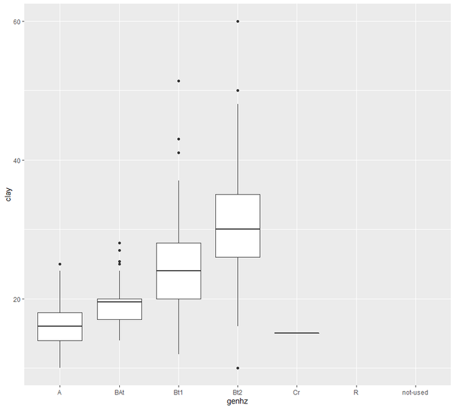
ggplot(h, (aes(x = genhz, y = clay))) +
geom_boxplot()
# QQ Plot for Clay
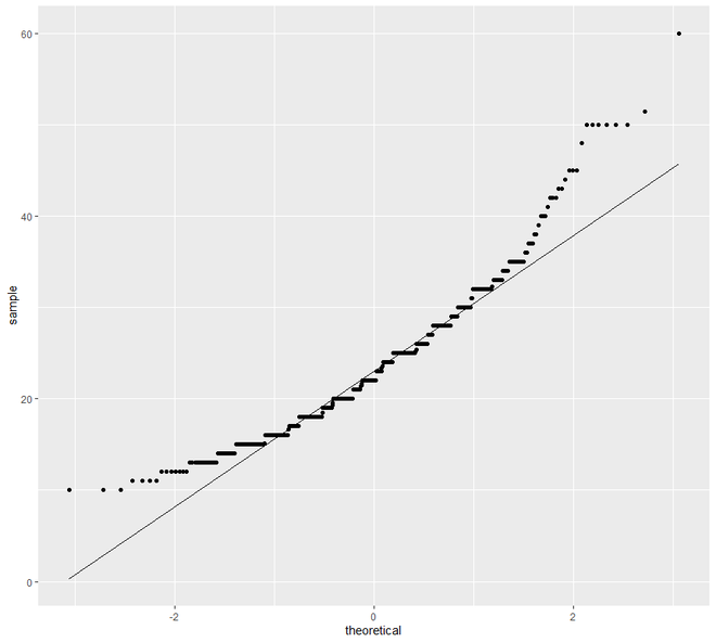
ggplot(h, aes(sample = clay)) +
geom_qq() +
geom_qq_line()R
# EDA
# Graphical Method
# Scatter and Line plot

# loading the required packages
library("ggplot2")
library(aqp)
library(soilDB)

# Load from the the loakercreek dataset
data("loafercreek")

# Construct generalized horizon designations
n <- c("A", "BAt", "Bt1", "Bt2", "Cr", "R")

# REGEX rules
p <- c("A", "BA|AB", "Bt|Bw", "Bt3|Bt4|2B|C",
       "Cr", "R")

# Compute genhz labels and add
# to loafercreek dataset
loafercreek$genhz <- generalize.hz(
                       loafercreek$hzname, n, p)

# Extract the horizon table
h <- horizons(loafercreek)

# Examine the matching of pairing
# of the genhz label to the hznames
table(h$genhz, h$hzname)

vars <- c("genhz", "clay", "total_frags_pct",
          "phfield", "effclass")
summary(h[, vars])

sort(unique(h$hzname))
h$hzname <- ifelse(h$hzname == "BT",
                   "Bt", h$hzname)

# graph
# scatter plot
ggplot(h, aes(x = clay, y = hzdepm)) +
  geom_point() +
  ylim(100, 0)

# line plot
ggplot(h, aes(y = clay, x = hzdepm,
                     group = peiid)) +
geom_line() + coord_flip() + xlim(100, 0)
输出:
> table(h$genhz, h$hzname)

           2BCt 2Bt1 2Bt2 2Bt3 2Bt4 2Bt5 2CB 2CBt 2Cr 2Crt 2R  A A1 A2 AB ABt Ad Ap  B BA BAt BC BCt Bt Bt1 Bt2 Bt3 Bt4 Bw Bw1 Bw2 Bw3  C
  A           0    0    0    0    0    0   0    0   0    0  0 97  7  7  0   0  1  1  0  0   0  0   0  0   0   0   0   0  0   0   0   0  0
  BAt         0    0    0    0    0    0   0    0   0    0  0  0  0  0  1   0  0  0  0 31   8  0   0  0   0   0   0   0  0   0   0   0  0
  Bt1         0    0    0    0    0    0   0    0   0    0  0  0  0  0  0   2  0  0  0  0   0  0   0  8  94  89   0   0 10   2   2   1  0
  Bt2         1    2    7    8    6    1   1    1   0    0  0  0  0  0  0   0  0  0  0  0   0  5  16  0   0   0  47   8  0   0   0   0  6
  Cr          0    0    0    0    0    0   0    0   4    2  0  0  0  0  0   0  0  0  0  0   0  0   0  0   0   0   0   0  0   0   0   0  0
  R           0    0    0    0    0    0   0    0   0    0  5  0  0  0  0   0  0  0  0  0   0  0   0  0   0   0   0   0  0   0   0   0  0
  not-used    0    0    0    0    0    0   0    0   0    0  0  0  0  0  0   0  0  0  1  0   0  0   0  0   0   0   0   0  0   0   0   0  0

           CBt Cd Cr Cr/R Crt H1 Oi  R Rt
  A          0  0  0    0   0  0  0  0  0
  BAt        0  0  0    0   0  0  0  0  0
  Bt1        0  0  0    0   0  0  0  0  0
  Bt2        6  1  0    0   0  0  0  0  0
  Cr         0  0 49    0  20  0  0  0  0
  R          0  0  0    1   0  0  0 41  1
  not-used   0  0  0    0   0  1 24  0  0

> summary(h[, vars])
      genhz          clay       total_frags_pct    phfield            effclass
 A       :113   Min.   :10.00   Min.   : 0.00   Min.   :4.90   very slight:  0
 BAt     : 40   1st Qu.:18.00   1st Qu.: 0.00   1st Qu.:6.00   slight     :  0
 Bt1     :208   Median :22.00   Median : 5.00   Median :6.30   strong     :  0
 Bt2     :116   Mean   :23.67   Mean   :14.18   Mean   :6.18   violent    :  0
 Cr      : 75   3rd Qu.:28.00   3rd Qu.:20.00   3rd Qu.:6.50   none       : 86
 R       : 48   Max.   :60.00   Max.   :95.00   Max.   :7.00   NA's       :540
 not-used: 26   NA's   :173                     NA's   :381

> sort(unique(h$hzname))
 [1] "2BCt" "2Bt1" "2Bt2" "2Bt3" "2Bt4" "2Bt5" "2CB"  "2CBt" "2Cr"  "2Crt" "2R"   "A"    "A1"   "A2"   "AB"   "ABt"  "Ad"   "Ap"   "B"
[20] "BA"   "BAt"  "BC"   "BCt"  "Bt"   "Bt1"  "Bt2"  "Bt3"  "Bt4"  "Bw"   "Bw1"  "Bw2"  "Bw3"  "C"    "CBt"  "Cd"   "Cr"   "Cr/R" "Crt"
[39] "H1"   "Oi"   "R"    "Rt"
现在继续进行 EDA。
EDA 中的描述性统计
对于描述性统计,为了在 R 中执行 EDA,我们将所有函数分为以下几类:
- 集中趋势的度量
- 分散测量
- 相关性
我们将尝试使用集中趋势度量下的函数来确定中点值。在本节中,我们将计算均值、中位数、众数和频率。
示例 1:现在查看此示例中的集中趋势度量。
R
# EDA
# Descriptive Statistics
# Measures of Central Tendency

#loading the required packages
library(aqp)
library(soilDB)

# Load from the the loakercreek dataset
data("loafercreek")

# Construct generalized horizon designations
n <- c("A", "BAt", "Bt1", "Bt2", "Cr", "R")

# REGEX rules
p <- c("A", "BA|AB", "Bt|Bw", "Bt3|Bt4|2B|C",
       "Cr", "R")

# Compute genhz labels and
# add to loafercreek dataset
loafercreek$genhz <- generalize.hz(
                       loafercreek$hzname,
                       n, p)

# Extract the horizon table
h <- horizons(loafercreek)

# Examine the matching of pairing
# of the genhz label to the hznames
table(h$genhz, h$hzname)

vars <- c("genhz", "clay", "total_frags_pct",
          "phfield", "effclass")
summary(h[, vars])

sort(unique(h$hzname))
h$hzname <- ifelse(h$hzname == "BT",
                   "Bt", h$hzname)

# first remove missing values
# and create a new vector
clay <- na.exclude(h$clay)

mean(clay)
median(clay)
sort(table(round(h$clay)),
     decreasing = TRUE)[1]
table(h$genhz)
# append the table with
# row and column sums
addmargins(table(h$genhz,
                 h$texcl))

# calculate the proportions
# relative to the rows, margin = 1
# calculates for rows, margin = 2 calculates
# for columns, margin = NULL calculates
# for total observations
round(prop.table(table(h$genhz, h$texture_class),
                 margin = 1) * 100)
knitr::kable(addmargins(table(h$genhz, h$texcl)))

aggregate(clay ~ genhz, data = h, mean)
aggregate(clay ~ genhz, data = h, median)
aggregate(clay ~ genhz, data = h, summary)
输出:
> mean(clay)
[1] 23.6713
> median(clay)
[1] 22
> sort(table(round(h$clay)), decreasing = TRUE)[1]
25
41
> table(h$genhz)

       A      BAt      Bt1      Bt2       Cr        R not-used
     113       40      208      116       75       48       26

> addmargins(table(h$genhz, h$texcl))

           cos   s  fs vfs lcos  ls lfs lvfs cosl  sl fsl vfsl   l sil  si scl  cl sicl  sc sic   c Sum
  A          0   0   0   0    0   0   0    0    0   6   0    0  78  27   0   0   0    0   0   0   0 111
  BAt        0   0   0   0    0   0   0    0    0   1   0    0  31   4   0   0   2    1   0   0   0  39
  Bt1        0   0   0   0    0   0   0    0    0   1   0    0 125  20   0   4  46    5   0   1   2 204
  Bt2        0   0   0   0    0   0   0    0    0   0   0    0  28   5   0   5  52    3   0   1  16 110
  Cr         0   0   0   0    0   0   0    0    0   0   0    0   0   0   0   0   0    0   0   0   1   1
  R          0   0   0   0    0   0   0    0    0   0   0    0   0   0   0   0   0    0   0   0   0   0
  not-used   0   0   0   0    0   0   0    0    0   0   0    0   0   0   0   0   1    0   0   0   0   1
  Sum        0   0   0   0    0   0   0    0    0   8   0    0 262  56   0   9 101    9   0   2  19 466

> round(prop.table(table(h$genhz, h$texture_class), margin = 1) * 100)

            br   c  cb  cl  gr   l  pg scl sic sicl sil  sl spm
  A          0   0   0   0   0  70   0   0   0    0  24   5   0
  BAt        0   0   0   5   0  79   0   0   0    3  10   3   0
  Bt1        0   1   0  23   0  61   0   2   0    2  10   0   0
  Bt2        0  14   1  46   2  25   1   4   1    3   4   0   0
  Cr        98   2   0   0   0   0   0   0   0    0   0   0   0
  R        100   0   0   0   0   0   0   0   0    0   0   0   0
  not-used   0   0   0   4   0   0   0   0   0    0   0   0  96

> knitr::kable(addmargins(table(h$genhz, h$texcl)))


|         | cos|  s| fs| vfs| lcos| ls| lfs| lvfs| cosl| sl| fsl| vfsl|   l| sil| si| scl|  cl| sicl| sc| sic|  c| Sum|
|:--------|---:|--:|--:|---:|----:|--:|---:|----:|----:|--:|---:|----:|---:|---:|--:|---:|---:|----:|--:|---:|--:|---:|
|A        |   0|  0|  0|   0|    0|  0|   0|    0|    0|  6|   0|    0|  78|  27|  0|   0|   0|    0|  0|   0|  0| 111|
|BAt      |   0|  0|  0|   0|    0|  0|   0|    0|    0|  1|   0|    0|  31|   4|  0|   0|   2|    1|  0|   0|  0|  39|
|Bt1      |   0|  0|  0|   0|    0|  0|   0|    0|    0|  1|   0|    0| 125|  20|  0|   4|  46|    5|  0|   1|  2| 204|
|Bt2      |   0|  0|  0|   0|    0|  0|   0|    0|    0|  0|   0|    0|  28|   5|  0|   5|  52|    3|  0|   1| 16| 110|
|Cr       |   0|  0|  0|   0|    0|  0|   0|    0|    0|  0|   0|    0|   0|   0|  0|   0|   0|    0|  0|   0|  1|   1|
|R        |   0|  0|  0|   0|    0|  0|   0|    0|    0|  0|   0|    0|   0|   0|  0|   0|   0|    0|  0|   0|  0|   0|
|not-used |   0|  0|  0|   0|    0|  0|   0|    0|    0|  0|   0|    0|   0|   0|  0|   0|   1|    0|  0|   0|  0|   1|
|Sum      |   0|  0|  0|   0|    0|  0|   0|    0|    0|  8|   0|    0| 262|  56|  0|   9| 101|    9|  0|   2| 19| 466|
> aggregate(clay ~ genhz, data = h, mean)
  genhz     clay
1     A 16.23113
2   BAt 19.53889
3   Bt1 24.14221
4   Bt2 31.35045
5    Cr 15.00000

> aggregate(clay ~ genhz, data = h, median)
  genhz clay
1     A 16.0
2   BAt 19.5
3   Bt1 24.0
4   Bt2 30.0
5    Cr 15.0

> aggregate(clay ~ genhz, data = h, summary)
  genhz clay.Min. clay.1st Qu. clay.Median clay.Mean clay.3rd Qu. clay.Max.
1     A  10.00000     14.00000    16.00000  16.23113     18.00000  25.00000
2   BAt  14.00000     17.00000    19.50000  19.53889     20.00000  28.00000
3   Bt1  12.00000     20.00000    24.00000  24.14221     28.00000  51.40000
4   Bt2  10.00000     26.00000    30.00000  31.35045     35.00000  60.00000
5 Cr 15.00000 15.00000 15.00000 15.00000 15.00000 15.00000现在我们将看到色散度量下的功能。在这个类别中,我们将确定中点附近的价差值。在这里,我们将计算方差、标准差、范围、四分位间距、方差系数和四分位数。
示例 2:
我们将在这个例子中看到分散的度量。
R
# EDA
# Descriptive Statistics
# Measures of Dispersion

# loading the packages
library(aqp)
library(soilDB)

# Load from the the loakercreek dataset
data("loafercreek")

# Construct generalized horizon designations
n <- c("A", "BAt", "Bt1", "Bt2", "Cr", "R")

# REGEX rules
p <- c("A", "BA|AB", "Bt|Bw", "Bt3|Bt4|2B|C",
       "Cr", "R")

# Compute genhz labels and add
# to loafercreek dataset
loafercreek$genhz <- generalize.hz(
                     loafercreek$hzname,
                       n, p)

# Extract the horizon table
h <- horizons(loafercreek)

# Examine the matching of pairing of
# the genhz label to the hznames
table(h$genhz, h$hzname)

vars <- c("genhz", "clay", "total_frags_pct",
          "phfield", "effclass")
summary(h[, vars])

sort(unique(h$hzname))
h$hzname <- ifelse(h$hzname == "BT",
                   "Bt", h$hzname)

# first remove missing values
# and create a new vector
clay <- na.exclude(h$clay)
var(h$clay, na.rm=TRUE)
sd(h$clay, na.rm = TRUE)
cv <- sd(clay) / mean(clay) * 100
cv
quantile(clay)
range(clay)
IQR(clay)
输出:
> var(h$clay, na.rm=TRUE)
[1] 64.89187

> sd(h$clay, na.rm = TRUE)
[1] 8.055549

> cv
[1] 34.03087

> quantile(clay)
  0%  25%  50%  75% 100%
  10   18   22   28   60

> range(clay)
[1] 10 60

> IQR(clay)
[1] 10现在我们将研究Correlation 。在这部分中,所有变量的所有计算相关系数值都列在表中作为相关矩阵。这为我们提供了一个量化的衡量标准,以指导我们的决策过程。
示例 3:
我们现在将在这个例子中看到相关性。
R
# EDA
# Descriptive Statistics
# Correlation

# loading the required packages
library(aqp)
library(soilDB)

# Load from the the loakercreek dataset
data("loafercreek")

# Construct generalized horizon designations
n <- c("A", "BAt", "Bt1", "Bt2", "Cr", "R")

# REGEX rules
p <- c("A", "BA|AB", "Bt|Bw", "Bt3|Bt4|2B|C",
       "Cr", "R")

# Compute genhz labels and add
# to loafercreek dataset
loafercreek$genhz <- generalize.hz(
                       loafercreek$hzname,
                     n, p)

# Extract the horizon table
h <- horizons(loafercreek)

# Examine the matching of pairing
# of the genhz label to the hznames
table(h$genhz, h$hzname)

vars <- c("genhz", "clay", "total_frags_pct",
          "phfield", "effclass")
summary(h[, vars])

sort(unique(h$hzname))
h$hzname <- ifelse(h$hzname == "BT",
                   "Bt", h$hzname)

# first remove missing values
# and create a new vector
clay <- na.exclude(h$clay)

# Compute the middle horizon depth
h$hzdepm <- (h$hzdepb + h$hzdept) / 2
vars <- c("hzdepm", "clay", "sand",
          "total_frags_pct", "phfield")
round(cor(h[, vars], use = "complete.obs"), 2)
输出:
hzdepm  clay  sand total_frags_pct phfield
hzdepm            1.00  0.59 -0.08            0.50   -0.03
clay              0.59  1.00 -0.17            0.28    0.13
sand             -0.08 -0.17  1.00           -0.05    0.12
total_frags_pct   0.50  0.28 -0.05            1.00   -0.16
phfield          -0.03  0.13  0.12           -0.16    1.00
因此,上述三个分类涉及 EDA 的描述性统计部分。现在我们将继续讨论表示 EDA 的图形方法。
EDA 中的图形方法
由于我们已经检查了我们的数据是否存在缺失值、明显错误和拼写错误,我们现在可以以图形方式检查我们的数据以执行 EDA。我们将在以下类别下看到图形表示:
- 分布
- 散点图和线图
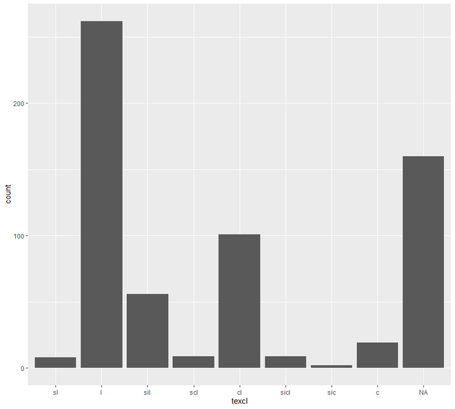
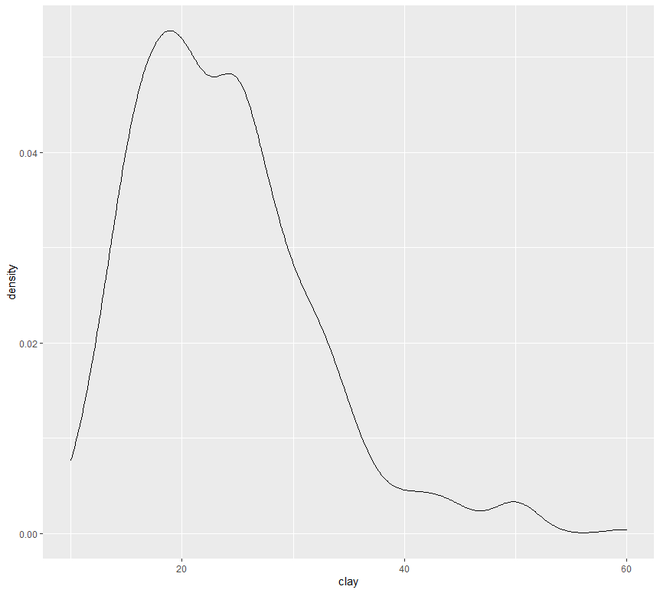
在分布下,我们将使用条形图、直方图、密度曲线、箱线图和 QQ 图来检查我们的数据。
示例 1:
在这个例子中,我们将看到如何使用分布图来检查 EDA 中的数据。
R
# EDA Graphical Method Distributions

# loading the required packages
library("ggplot2")
library(aqp)
library(soilDB)

# Load from the the loakercreek dataset
data("loafercreek")

# Construct generalized horizon designations
n <- c("A", "BAt", "Bt1", "Bt2", "Cr", "R")

# REGEX rules
p <- c("A", "BA|AB", "Bt|Bw", "Bt3|Bt4|2B|C",
       "Cr", "R")

# Compute genhz labels and add
# to loafercreek dataset
loafercreek$genhz <- generalize.hz(
                       loafercreek$hzname, n, p)

# Extract the horizon table
h <- horizons(loafercreek)

# Examine the matching of pairing
# of the genhz label to the hznames
table(h$genhz, h$hzname)

vars <- c("genhz", "clay", "total_frags_pct",
          "phfield", "effclass")
summary(h[, vars])

sort(unique(h$hzname))
h$hzname <- ifelse(h$hzname == "BT",
                   "Bt", h$hzname)

# graphs
# bar plot
ggplot(h, aes(x = texcl)) +geom_bar()

# histogram
ggplot(h, aes(x = clay)) +
  geom_histogram(bins = nclass.Sturges(h$clay))

# density curve
ggplot(h, aes(x = clay)) + geom_density()

# box plot
ggplot(h, (aes(x = genhz, y = clay))) +
geom_boxplot()

# QQ Plot for Clay
ggplot(h, aes(sample = clay)) +
geom_qq() +
geom_qq_line()
输出:

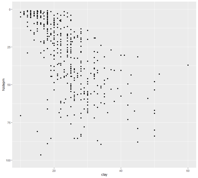
现在我们将继续进行散点图和线图。在这个类别中,我们将看到两种类型的绘图,散点图和线图。一个区间或比率变量对变量的绘图点称为散点图。
示例 2:
我们现在将了解如何使用散点图和折线图来检查我们的数据。
R
# EDA
# Graphical Method
# Scatter and Line plot
# loading the required packages
library("ggplot2")
library(aqp)
library(soilDB)
# Load from the the loakercreek dataset
data("loafercreek")
# Construct generalized horizon designations
n <- c("A", "BAt", "Bt1", "Bt2", "Cr", "R")
# REGEX rules
p <- c("A", "BA|AB", "Bt|Bw", "Bt3|Bt4|2B|C",
"Cr", "R")
# Compute genhz labels and add
# to loafercreek dataset
loafercreek$genhz <- generalize.hz(
loafercreek$hzname, n, p)
# Extract the horizon table
h <- horizons(loafercreek)
# Examine the matching of pairing
# of the genhz label to the hznames
table(h$genhz, h$hzname)
vars <- c("genhz", "clay", "total_frags_pct",
"phfield", "effclass")
summary(h[, vars])
sort(unique(h$hzname))
h$hzname <- ifelse(h$hzname == "BT",
"Bt", h$hzname)
# graph
# scatter plot
ggplot(h, aes(x = clay, y = hzdepm)) +
geom_point() +
ylim(100, 0)
# line plot
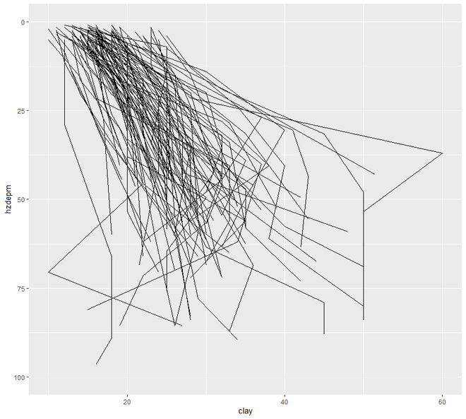
ggplot(h, aes(y = clay, x = hzdepm,
group = peiid)) +
geom_line() + coord_flip() + xlim(100, 0)
输出: