连续核卷积

连续内核卷积是由阿姆斯特丹 Verije 大学的研究人员与阿姆斯特丹大学合作在一篇题为“ CKConv：Continuous Kernel Convolution For Sequential Data ”的论文中提出的。其背后的动机是提出一个模型，该模型使用卷积神经网络和循环神经网络的特性来处理长序列的图像数据。

卷积运算

设 x ∶R → R ^N _^c和 ψ ∶ R → R ^N _^c是 R 上的向量值信号和核，使得 x = {x _c } ^Nc和 ψ = {ψ _c } N _C c=1。卷积操作可以定义为：

$(x * \psi)(t) = \sum_{c=1}^{N_c} \int_\mathbb{R} x_c(\tau)\psi_c(t-\tau)d\tau$

然而，实际上输入信号 x 是从采样中收集的。因此，输入信号和卷积可以定义为

输入信号： $\chi = {x(\tau )}_{\tau=0}^{N_x}$
卷积： $\kappa = {\psi(\tau)}_{\tau=0}^{N_x}$

以t为中心的方程由下式给出：

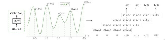
$(\chi * \psi)(t) = \sum_{c=1}^{N_c} \sum_{\tau = 0}^{t}x_c\left ( \tau \right )\psi_c\left ( t-\tau \right )$

现在对于连续核卷积，我们将使用卷积核 ψ 作为参数化在一个名为MLP ^ψ的小型神经网络上的连续函数。它以(t−τ )作为输入并输出卷积核在那个位置ψ(t−τ ) 的值。连续核可以由以下公式表示：

$(\chi * \psi)(t) = \sum_{c=1}^{N_c} \sum_{\tau = 0}^{t}x_c\left ( \tau \right )MLP^{\psi_c}\left ( t-\tau \right )$

如果采样因子与训练采样因子不同，那么我们可以通过以下方式进行卷积运算：

$(\chi * \psi)(t)_{sr2} \approx \frac{sr2}{sr1}(\chi * \psi)(t)_{sr1}$

经常单位

对于输入序列

$\chi = {x(\tau )}_{\tau=0}^{N_x}$ .循环单位由下式给出：

$h(\tau) = \sigma(Wh(\tau-1) + U_x(\tau))$

$\tilde{y} (\tau) = softmax (Vh(\tau))$

其中 U、W、V 是单元的输入到隐藏、隐藏到隐藏和隐藏到输出的连接。 h(τ)、y~(τ) 描述了隐藏表示和时间步长 τ 的输出，σ 表示逐点非线性。

现在，我们将上述方程展开为 t 步：

$h(t) = W^{t+1}h(-1) + \sum_{\tau =0 } ^{t} W^{\tau} U x(t - \tau)$

其中 h(−1) 是隐藏表示的初始状态。 h(t) 也可以用以下方式表示：

$x =[x(0), x(1), x(2) .....x(t-1),x(t)] \\ \psi =[U, WU, .... W^{t-1}U, W^{t}U] \\ h(t) = \sum_{\tau =0 }^{t}x(\tau)\psi(t-\tau) + \sum_{\tau =0 }^{t}x(t - \tau)\psi(\tau)$

上述等式为我们提供了以下结论：

RNN 中的梯度消失和梯度爆炸问题是由过去的 x(t-τ) τ 项乘以有效卷积权重 ψ(τ)=W ^τ U 引起的。
线性循环单元可以定义为输入和指数卷积函数的卷积。

MLP 连续内核

令 {∆t _i =(t − τ _i )} ^N i=0 是一个相对位置序列。卷积核 MLP _ψ由传统的 L 层神经网络参数化：

MLP

$h^{(1)}(\Delta \tau_i ) = \sigma\left ( w^{1} \Delta \tau_i + b^{(1)} \right ) \\ h^{(1)}(\Delta \tau_i ) = \sigma\left ( W^{l} * h* (l-1) \Delta \tau_i + b^{(1)} \right ) \\ \psi(\Delta \tau_i) = W^{(L)} * h{(L-1)} (\Delta \tau_i) + b^{(L)}$

在哪里，

$\sigma$ 用于添加非线性，例如 ReLU。

执行

在这个实现中，我们将在 sMNIST 数据集上训练 CKconv 模型，对于这个实现，我们将使用谷歌提供给我们的 colaboratory。

Python3

# code credits: https://github.com/dwromero/ckconv
# first, we need to clone the ckconv repository from Github
! git clone https://github.com/dwromero/ckconv
 
# Now, we need to change the pwd to ckconv directory
cd ckconv
 
# Before actually train the model,
# we need to first install the required modules and libraries
! pip install -r requirements.txt
 
# if the above command fails, please make sure that following modules installed using
# command below
pip install ml-collections torchaudio mkl-random sktime wandb
 
# Now to train the model on sMNIst dataset, run the following commands
! python run_experiment.py --config.batch_size=64 --config.clip=0 \
--config.dataset=MNIST --config.device=cuda --config.dropout=0.1 \
--config.dropout_in=0.1 --config.epochs=200 --config.kernelnet_activation_function=Sine \
--config.kernelnet_no_hidden=32 --config.kernelnet_norm_type=LayerNorm \
--config.kernelnet_omega_0=31.09195739463897 --config.lr=0.001 --config.model=CKCNN \
--config.no_blocks=2 --config.no_hidden=30 --config.optimizer=Adam \
--config.permuted=False --config.sched_decay_factor=5  --config.sched_patience=20 \
--config.scheduler=plateau

以下是CKCNN在sMNIST数据上的上述训练结果：

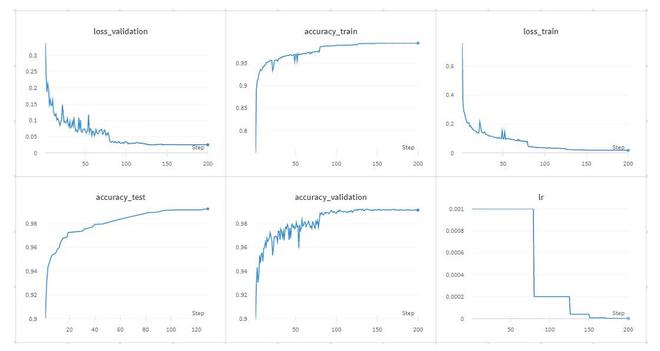
CkConv 训练结果

结论

Ckconv 能够轻松处理非常复杂的非线性函数。
与 RNN 不同，CKConvs 不依赖任何形式的递归来考虑大内存范围，并且具有全局长期依赖性。
CKCNN 不使用时间反向传播（BPTT）。因此，可以并行训练 CKCNN。
CKCNN 也可以部署在除训练分辨率以外的分辨率。

参考：

CKConv 论文