MATLAB中高斯滤波器的拉普拉斯算子

拉普拉斯滤波器用于检测图像中的边缘。但它比嘈杂的图像有一个缺点。它放大了图像中的噪声。因此，首先，我们在噪声图像上使用高斯滤波器对其进行平滑处理，然后使用拉普拉斯滤波器进行边缘检测。

处理没有高斯滤波器的嘈杂图像：

使用的函数

• imread() 用于图像读取。
• rgb2gray( ) 用于获取灰度图像。
• conv2( ) 用于卷积。
• imtool( )函数用于显示图像。

例子：

Matlab

% Read the image in MatLab
j=imread("logo.png");
 
% Convert the image in gray scale.
j1=rgb2gray(j);
 
% Generate the noise of size equal to gray image.
n=25*randn(size(j1));
 
% Generate noisy image by adding noise to the grayscale image.
j2=n+double(j1);
 
% Display the original color image.
imtool(j,[]);
 
% Display the gray image.
imtool(j1,[]);
 
% Display the noisy image.
imtool(j2,[]);
 
% Define the Laplacian Filter.
Lap=[0 -1 0; -1 4 -1; 0 -1 0];
 
% Convolve the noisy image with Laplacian filter.
j3=conv2(j2, Lap, 'same');
 
% Display the resultant image.
imtool(abs(j3), []);

输出：

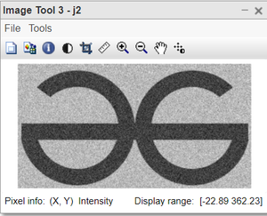
图：输入噪声图像

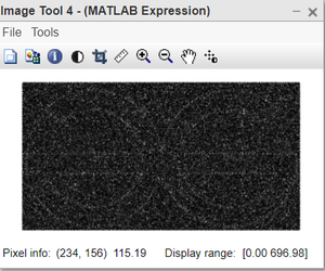
图：边缘检测图像

代码说明：

• j=imread(“logo.png”);这一行读取 MatLab 中的图像
  图像的扩展名可以是任何东西，例如 jfif、png、jpg、jpeg 等。
• j1=rgb2gray(j);这条线将图像转换为灰度，我们避免处理彩色图像。
  该函数只接受一个参数并返回灰度图像。
• n=25*randn(大小(j1));这条线产生大小等于灰度图像的噪声。
  高斯噪声本质上是加性的，因此直接使用 + 进行添加。
• j2=n+双（j1）；此行通过向灰度图像添加噪声来生成噪声图像。
• imtool(j,[]);此行显示原始彩色图像。
• imtool(j1,[]);此行显示灰度图像。
• imtool(j2,[]);这条线显示嘈杂的图像。
• 圈=[0 -1 0; -1 4 -1; 0 -1 0];这行代码定义了拉普拉斯滤波器。
• j3=conv2(j2, Lap, 'same');这条线用拉普拉斯滤波器对噪声图像进行卷积。
  conv2(·) 执行卷积。它需要3个参数。 'same' 确保结果与输入图像的大小相同。
• imtool(abs(j3), []);此行显示生成的图像。

使用 LOG 处理嘈杂的图像：

图像的对数变换是灰度图像变换的一种。图像的对数变换意味着用其对数值替换图像中存在的所有像素值。对数变换用于图像增强，因为与更高的像素值相比，它会扩展图像的暗像素。

例子：

MATLAB

% Read the image in MatLab
j=imread("logo.png");
 
% Convert the image in gray scale.
j1=rgb2gray(j);
 
% Generate the noise of size equal to gray image.
n=25*randn(size(j1));
 
% Generate noisy image by adding
% noise to the grayscale image.
j2=n+double(j1);
 
% Display the original color image.
imtool(j,[]);
 
% Display the gray image.
imtool(j1,[]);
 
% Display the noisy image.
imtool(j2,[]);
 
% Create the gaussian Filter.
Gaussian=fspecial('gaussian', 5, 1);
 
% Define the Laplacian Filter.
Lap=[0 -1 0; -1 4 -1; 0 -1 0];
 
% Convolve the noisy image
% with Gaussian Filter first.
j4=conv2(j2, Gaussian, 'same');
 
% Convolve the resultant
% image with Laplacian filter.
j5=conv2(j4, Lap, 'same');
 
% Display the Gaussian of noisy_image.
imtool(j4,[]);
 
% Display the Laplacian of
% Gaussian resultant image.
imtool(j5,[]);

输出：

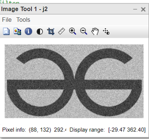
图：输入噪声图像

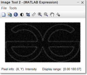
图：边缘检测图像

代码说明：

• j=imread(“logo.png”);这一行读取 MatLab 中的图像
  图像存储在变量 j 中。
• j1=rgb2gray(j);这条线将图像转换为灰度，我们避免处理彩色图像。
  j1 是灰度图像，j 是彩色图像。
• n=25*randn(大小(j1));这条线产生大小等于灰度图像的噪声。
  创建随机高斯噪声。
• j2=n+双（j1）；此行通过向灰度图像添加噪声来生成噪声图像。
  由于高斯噪声的成瘾性，它被直接添加到图像中。
• 高斯=fspecial('高斯', 5, 1);这条线创建了高斯滤波器。
  5 是均值，1 是高斯滤波器的方差。
• 圈=[0 -1 0; -1 4 -1; 0 -1 0];这行代码定义了拉普拉斯滤波器。
• j4=conv2(j2, 高斯, '相同');这条线首先用高斯滤波器对噪声图像进行卷积。
• j5=conv2(j4, Lap, 'same');这条线用拉普拉斯滤波器对结果图像进行卷积。
• imtool(j4,[]);这条线显示了noisy_image 的高斯。
• imtool(j5,[]);此行显示高斯结果图像的拉普拉斯算子。