销售预测 - Python

预测预测是使用过去值和许多其他因素来预测未来值。在本教程中，我们将使用 Keras 函数式 API 创建一个销售预测模型。

销售预测

它使用过去的销售额、季节性、庆祝活动、经济状况等数据来确定当前或未来的销售额。

因此，该模型将在提供一组特定输入后预测某一天的销售额。

在这个模型中，8 个参数被用作输入：

1. 过去 7 天的销售
2. 一周中的天
3. 日期 - 日期被转换为 3 个不同的输入
4. 季节
5. 节日与否
6. 去年同一天的销售额

它是如何工作的？

首先，所有输入都经过预处理，以便机器可以理解。这是一个基于监督学习的线性回归模型，因此输出将与输入一起提供。然后将输入与所需的输出一起输入模型。该模型将绘制（学习）输入和输出之间的关系（函数）。然后使用此函数或关系来预测一组特定输入的输出。在这种情况下，输入参数如日期和以前的销售额被标记为输入，而销售额被标记为输出。该模型将预测 0 到 1 之间的数字，因为最后一层使用了 sigmoid函数。这个输出可以乘以一个特定的数字（在这种情况下，最大销售额），这将是我们某一天对应的销售额。然后将此输出作为输入提供以计算第二天的销售数据。这个步骤循环将一直持续到某个日期到来。

所需的包和安装

1. 麻木的
2. 熊猫
3. 凯拉斯
4. 张量流
5. 文件
6. matplotlib.pyplot

Python3

import pandas as pd                     # to extract data from dataset(.csv file)
import csv                              #used to read and write to csv files
import numpy as np                      #used to convert input into numpy arrays to be fed to the model
import matplotlib.pyplot as plt         #to plot/visualize sales data and sales forecasting
import tensorflow as tf                 # acts as the framework upon which this model is built
from tensorflow import keras            #defines layers and functions in the model
 
#here the csv file has been copied into three lists to allow better availability
list_row,date,traffic = get_data('/home/abh/Documents/Python/Untitled Folder/Sales_dataset')

已将外部库的使用保持在最低限度以提供更简单的界面，您可以将本教程中使用的函数替换为已建立的库中已存在的函数。

5年销售数据的原始数据集：

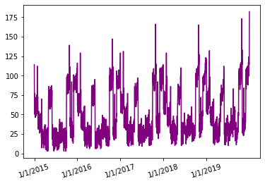
2015年1月至2019年12月销售数据

如您所见，每年的销售数据似乎都遵循类似的模式，并且在 5 年的时间范围内，销售峰值似乎随着时间的推移而增加。

在这 5 年的时间范围内，前 4 年将用于训练模型，最后一年将用作测试集。

现在，一些辅助函数用于处理数据集并创建所需形状和大小的输入。它们如下：

1. get_data – 用于使用指向其位置的路径加载数据集。
2. date_to_day – 为每一天提供一天。例如 - 2/2/16 是星期六，9/5/15 是星期一。
3. date_to_enc – 将数据编码为 one-hot 向量，这为模型提供了更好的学习机会。

这些函数和一些其他函数的所有属性在这里无法解释，因为这会花费太多时间。如果您想查看整个代码，请访问此链接。

预处理：

最初，数据集只有两列：日期和流量（销售额）。

在添加不同的列和值的处理/规范化之后，数据包含所有这些值。

1. 日期
2. 交通
3. 假期与否
4. 日

所有这些参数都必须转换成机器可以理解的形式，这将使用下面的这个函数来完成。

它没有将日期、月份和年份保留为单个实体，而是分为三个不同的输入。原因是这些输入中的年份参数大部分时间都是相同的，这将导致模型变得自满，即它将开始过度拟合当前数据集。为了增加不同输入日期之间的可变性，分别标记了日期和月份。下面的函数convert() 将创建六个列表并向它们附加适当的输入。这就是 2015 年到 2019 年的编码方式：

{2015: array([1., 0., 0., 0., 0.], dtype=float32), 2016: array([0., 1., 0., 0., 0.], dtype= float32), 2017: array([0., 0., 1., 0., 0.], dtype=float32), 2018: array([0., 0., 0., 1., 0.], dtype=float32), 2019: array([0., 0., 0., 0., 1.], dtype=float32)

它们中的每一个都是一个长度为 5 的 numpy 数组，其中 1 和 0 表示其值

蟒蛇3

def conversion(week,days,months,years,list_row):
  #lists have been defined to hold different inputs
  inp_day = []
  inp_mon = []
  inp_year = []
  inp_week=[]
  inp_hol=[]
  out = []
  #converts the days of a week(monday,sunday,etc.) into one hot vectors and stores them as a dictionary
  week1 = number_to_one_hot(week)
  #list_row contains primary inputs
  for row in list_row:
        #Filter out date from list_row
        d = row[0]
        #the date was split into three values date, month and year.
        d_split=d.split('/')
        if d_split[2]==str(year_all[0]):
          #prevents use of the first year data to ensure each input contains previous year data as well.
          continue
        #encode the three parameters of date into one hot vectors using date_to_enc function.
        d1,m1,y1 = date_to_enc(d,days,months,years) #days, months and years and dictionaries containing the one hot encoding of each date,month and year.
        inp_day.append(d1) #append date into date input
        inp_mon.append(m1) #append month into month input
        inp_year.append(y1) #append year into year input
        week2 = week1[row[3]] #the day column from list_is converted into its one-hot representation and saved into week2 variable
        inp_week.append(week2)# it is now appended into week input.
        inp_hol.append([row[2]])#specifies whether the day is a holiday or not
        t1 = row[1] #row[1] contains the traffic/sales value for a specific date
        out.append(t1) #append t1(traffic value) into a list out
  return inp_day,inp_mon,inp_year,inp_week,inp_hol,out #all the processed inputs are returned
 
inp_day,inp_mon,inp_year,inp_week,inp_hol,out = conversion(week,days,months,years,list_train)
#all of the inputs must be converted into numpy arrays to be fed into the model
inp_day = np.array(inp_day)
inp_mon = np.array(inp_mon)
inp_year = np.array(inp_year)
inp_week = np.array(inp_week)
inp_hol = np.array(inp_hol)

我们现在将处理剩余的一些其他输入，使用所有这些参数的原因是为了提高模型的效率，您可以尝试删除或添加一些输入。

过去 7 天的销售数据作为输入传递，以创建销售数据的趋势，这样预测值不会同样完全随机，还提供了上一年同一天的销售数据。

以下函数(other_inputs) 处理三个输入：

• 过去7天的销售数据
• 上年同日的销售数据
• 季节性 - 添加季节性以标记夏季销售等趋势。

蟒蛇3

def other_inputs(season,list_row):
  #lists to hold all the inputs
  inp7=[]
  inp_prev=[]
  inp_sess=[]
  count=0 #count variable will be used to keep track of the index of current row in order to access the traffic values of past seven days.
  for row in list_row:
    ind = count
    count=count+1
    d = row[0] #date was copied to variable d
    d_split=d.split('/')
    if d_split[2]==str(year_all[0]):
      #preventing use of the first year in the data
      continue
    sess = cur_season(season,d) #assigning a season to to the current date
    inp_sess.append(sess) #appending sess variable to an input list
    t7=[] #temporary list to hold seven sales value
    t_prev=[] #temporary list to hold the previous year sales value
    t_prev.append(list_row[ind-365][1]) #accessing the sales value from one year back and appending them
    for j in range(0,7):
        t7.append(list_row[ind-j-1][1]) #appending the last seven days sales value
    inp7.append(t7)
    inp_prev.append(t_prev)
  return inp7,inp_prev,inp_sess
 
inp7,inp_prev,inp_sess = other_inputs(season,list_train)
inp7 = np.array(inp7)
inp7= inp7.reshape(inp7.shape[0],inp7.shape[1],1)
inp_prev = np.array(inp_prev)
inp_sess = np.array(inp_sess)

这么多输入背后的原因是，如果将所有这些组合成一个数组，它将具有不同长度的不同行或列。这样的数组不能作为输入。

将所有值线性排列在单个数组中会导致模型具有高损失。

线性排列会导致模型泛化，因为连续输入之间的差异不会太大，这将导致学习受限，降低模型的准确性。

定义模型

八个独立的输入被处理并连接成一个层并传递给模型。

最终输入如下：

1. 日期
2. 月
3. 年
4. 日
5. 前 7 天销售
6. 前一年的销售额
7. 季节
8. 假期与否

这里在大多数层中，我使用了 5 个单元作为输出形状，您可以进一步试验它以提高模型的效率。

Python

from tensorflow.keras.models import Model
from tensorflow.keras.layers import Input, Dense,LSTM,Flatten
from tensorflow.keras.layers import concatenate
#an Input variable is made from every input array
input_day = Input(shape=(inp_day.shape[1],),name = 'input_day')
input_mon = Input(shape=(inp_mon.shape[1],),name = 'input_mon')
input_year = Input(shape=(inp_year.shape[1],),name = 'input_year')
input_week = Input(shape=(inp_week.shape[1],),name = 'input_week')
input_hol = Input(shape=(inp_hol.shape[1],),name = 'input_hol')
input_day7 = Input(shape=(inp7.shape[1],inp7.shape[2]),name = 'input_day7')
input_day_prev = Input(shape=(inp_prev.shape[1],),name = 'input_day_prev')
input_day_sess = Input(shape=(inp_sess.shape[1],),name = 'input_day_sess')
# The model is quite straight-forward, all inputs were inserted into a dense layer with 5 units and 'relu' as activation function
x1 = Dense(5, activation='relu')(input_day)
x2 = Dense(5, activation='relu')(input_mon)
x3 = Dense(5, activation='relu')(input_year)
x4 = Dense(5, activation='relu')(input_week)
x5 = Dense(5, activation='relu')(input_hol)
x_6 = Dense(5, activation='relu')(input_day7)
x__6 = LSTM(5,return_sequences=True)(x_6) # LSTM is used to remember the importance of each day from the seven days data
x6 = Flatten()(x__10) # done to make the shape compatible to other inputs as LSTM outputs a three dimensional tensor
x7 = Dense(5, activation='relu')(input_day_prev)
x8 = Dense(5, activation='relu')(input_day_sess)
c = concatenate([x1,x2,x3,x4,x5,x6,x7,x8]) # all inputs are concatenated into one
layer1 = Dense(64,activation='relu')(c)
outputs = Dense(1, activation='sigmoid')(layer1) # a single output is produced with value ranging between 0-1.
# now the model is initialized and created as well
model = Model(inputs=[input_day,input_mon,input_year,input_week,input_hol,input_day7,input_day_prev,input_day_sess], outputs=outputs)
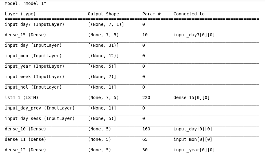
model.summary() # used to draw a summary(diagram) of the model

型号概要：

使用 RMSprop 编译模型：

RMSprop 擅长处理随机分布，因此在这里使用它。

蟒蛇3

from tensorflow.keras.optimizers import RMSprop
 
model.compile(loss=['mean_squared_error'],
              optimizer = 'adam',
              metrics = ['acc'] #while accuracy is used as a metrics here it will remain zero as this is no classification model
              )                  # linear regression models are best gauged by their loss value

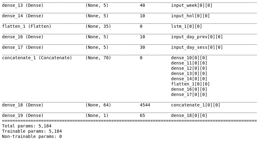
在数据集上拟合模型：

现在模型将输入输入和输出数据，这是最后一步，现在我们的模型将能够预测销售数据。

蟒蛇3

history = model.fit(
           x = [inp_day,inp_mon,inp_year,inp_week,inp_hol,inp7,inp_prev,inp_sess],
           y = out,
           batch_size=16,
           steps_per_epoch=50,
           epochs = 15,
           verbose=1,
           shuffle =False
           )
#all the inputs were fed into the model and the training was completed

输出：

现在，为了测试模型， input() 接受输入并将其转换为适当的形式：

蟒蛇3

def input(date):
    d1,d2,d3 = date_to_enc(date,days,months,years)   #separate date into three parameters
    print('date=',date)
    d1 = np.array([d1])                        
    d2 = np.array([d2])
    d3 = np.array([d3])
    week1 = number_to_one_hot(week)        #defining one hot vector to encode days of a week
    week2 = week1[day[date]]
    week2=np.array([week2])
    //appeding a column for holiday(0-not holiday, 1- holiday)
    if date in holiday:
        h=1
        #print('holiday')
    else:
        h=0
        #print("no holiday")
    h = np.array([h])
    sess = cur_season(season,date)        #getting seasonality data from cur_season function
    sess = np.array([sess])                            
    return d1,d2,d3,week2,h,sess

预测销售数据不是我们在这里的目的，所以让我们继续预测工作。

销售预测

定义forecast_testing函数来预测从提供日期起一年后的销售数据：

该函数的工作原理如下：

• 需要一个日期作为输入来预测从一年前到上述日期的销售数据
• 然后，我们访问上一年当日的销售数据和前 7 天的销售数据。
• 然后，使用这些作为输入预测新值，然后在 7 天的值中删除第一天，并将预测输出添加为下一个预测的输入

例如：我们需要预测到 31/12/2019 的一年

• 首先，记录 31/12/2018（一年前）的日期，以及 (25/12/2018 – 31/12/2018) 的 7 天销售额
• 然后收集一年前的销售数据，即 31/12/2017
• 使用这些作为与其他输入的输入，预测第一个销售数据（即 1/1/2019）
• 然后删除 24/12/2018 销售数据并添加 1/1/2019 预测销售额。重复此循环，直到预测 31/12/2019 的销售数据。

因此，以前的输出用作输入。

蟒蛇3

def forecast_testing(date):
    maxj = max(traffic) # determines the maximum sales value in order to normalize or return the data to its original form
    out=[]
    count=-1
    ind=0
    for i in list_row:
        count =count+1
        if i[0]==date: #identify the index of the data in list
            ind = count
    t7=[]
    t_prev=[]
    t_prev.append(list_row[ind-365][1]) #previous year data
    # for the first input, sales data of last seven days will be taken from training data
    for j in range(0,7):
          t7.append(list_row[ind-j-365][1])
    result=[] # list to store the output and values
    count=0
    for i in list_date[ind-364:ind+2]:
        d1,d2,d3,week2,h,sess = input(i) # using input function to process input values into numpy arrays
        t_7 = np.array([t7]) # converting the data into a numpy array
        t_7 = t_7.reshape(1,7,1)
        # extracting and processing the previous year sales value
        t_prev=[]
        t_prev.append(list_row[ind-730+count][1])
        t_prev = np.array([t_prev])
        #predicting value for output
        y_out = model.predict([d1,d2,d3,week2,h,t_7,t_prev,sess])
        #output and multiply the max value to the output value to increase its range from 0-1
        print(y_out[0][0]*maxj)
        t7.pop(0) #delete the first value from the last seven days value
        t7.append(y_out[0][0]) # append the output as input for the seven days data
        result.append(y_out[0][0]*maxj) # append the output value to the result list
        count=count+1
    return result

运行预测测试函数，返回包含该年所有销售数据的列表

结果 = 预测测试（'31/12/2019'，日期）

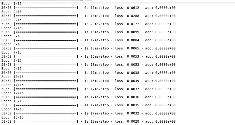
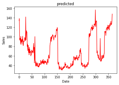
用于测试模型性能的预测值和实际值的图表

蟒蛇3

plt.plot(result,color='red',label='predicted')
plt.plot(test_sales,color='purple',label="actual")
plt.xlabel("Date")
plt.ylabel("Sales")
leg = plt.legend()
plt.show()

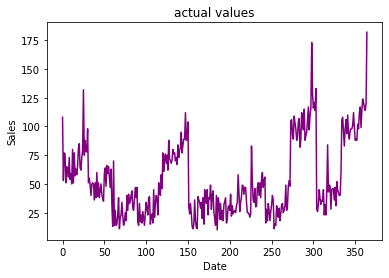
2019 年 1 月 1 日至 2019 年 12 月 31 日的实际值

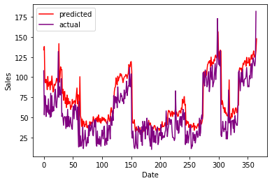
预测值与实际值的比较

如您所见，预测值和实际值非常接近，这证明了我们模型的效率。以上文章如有错误或改进的可能，欢迎在评论区提出。