Python – 统计学中的麦克斯韦分布

scipy.stats.maxwell()是麦克斯韦（第二类帕累托）连续随机变量。它作为rv_continuous 类的实例继承自泛型方法。它使用特定于此特定发行版的详细信息来完成方法。

参数 ：

q : lower and upper tail probability
x : quantiles
loc : [optional]location parameter. Default = 0
scale : [optional]scale parameter. Default = 1
size : [tuple of ints, optional] shape or random variates.
moments : [optional] composed of letters [‘mvsk’]; ‘m’ = mean, ‘v’ = variance, ‘s’ = Fisher’s skew and ‘k’ = Fisher’s kurtosis. (default = ‘mv’).

Results : Maxwell continuous random variable

代码#1：创建麦克斯韦连续随机变量

# importing library
  
from scipy.stats import maxwell  
    
numargs = maxwell.numargs 
a, b = 4.32, 3.18
rv = maxwell(a, b) 
    
print ("RV : \n", rv)  

输出 ：

RV : 
 scipy.stats._distn_infrastructure.rv_frozen object at 0x000002A9D66DEC88

代码 #2：麦克斯韦连续变量和概率分布

import numpy as np 
quantile = np.arange (0.01, 1, 0.1) 
  
# Random Variates 
R = maxwell.rvs(a, b) 
print ("Random Variates : \n", R) 
  
# PDF 
R = maxwell.pdf(a, b, quantile) 
print ("\nProbability Distribution : \n", R) 

输出 ：

Random Variates : 
 8.999401872992793

Probability Distribution : 
 [0.00000000e+00 3.70579394e-21 4.46576264e-05 4.02803131e-02
 3.15216150e-01 6.42768234e-01 7.96800760e-01 7.98281605e-01
 7.24720266e-01 6.27826999e-01]

代码#3：图形表示。

import numpy as np 
import matplotlib.pyplot as plt 
     
distribution = np.linspace(0, np.minimum(rv.dist.b, 3)) 
print("Distribution : \n", distribution) 
     
plot = plt.plot(distribution, rv.pdf(distribution)) 

输出 ：

Distribution : 
 [0.         0.06122449 0.12244898 0.18367347 0.24489796 0.30612245
 0.36734694 0.42857143 0.48979592 0.55102041 0.6122449  0.67346939
 0.73469388 0.79591837 0.85714286 0.91836735 0.97959184 1.04081633
 1.10204082 1.16326531 1.2244898  1.28571429 1.34693878 1.40816327
 1.46938776 1.53061224 1.59183673 1.65306122 1.71428571 1.7755102
 1.83673469 1.89795918 1.95918367 2.02040816 2.08163265 2.14285714
 2.20408163 2.26530612 2.32653061 2.3877551  2.44897959 2.51020408
 2.57142857 2.63265306 2.69387755 2.75510204 2.81632653 2.87755102
 2.93877551 3.        ]
 

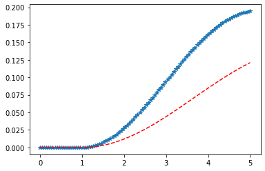
代码#4：改变位置参数

import matplotlib.pyplot as plt 
import numpy as np 
     
x = np.linspace(0, 5, 100) 
     
# Varying positional arguments 
y1 = maxwell .pdf(x, 1, 3) 
y2 = maxwell .pdf(x, 1, 4) 
plt.plot(x, y1, "*", x, y2, "r--") 

输出 ：