毫升 |使用 TensorFlow 进行逻辑回归
先决条件:了解逻辑回归和 TensorFlow。
逻辑回归的简要总结:
逻辑回归是机器学习中常用的分类算法。它允许通过从一组给定的标记数据中学习关系来将数据分类为离散的类。它从给定的数据集中学习线性关系,然后以 Sigmoid函数的形式引入非线性。
在逻辑回归的情况下,假设是一条直线的 Sigmoid,即 在哪里
在哪里
其中向量w代表权重,标量b代表模型的偏差。
让我们可视化 Sigmoid函数——
import numpy as np
import matplotlib.pyplot as plt

def sigmoid(z):
    return 1 / (1 + np.exp( - z))

plt.plot(np.arange(-5, 5, 0.1), sigmoid(np.arange(-5, 5, 0.1)))
plt.title('Visualization of the Sigmoid Function')

plt.show()
输出: 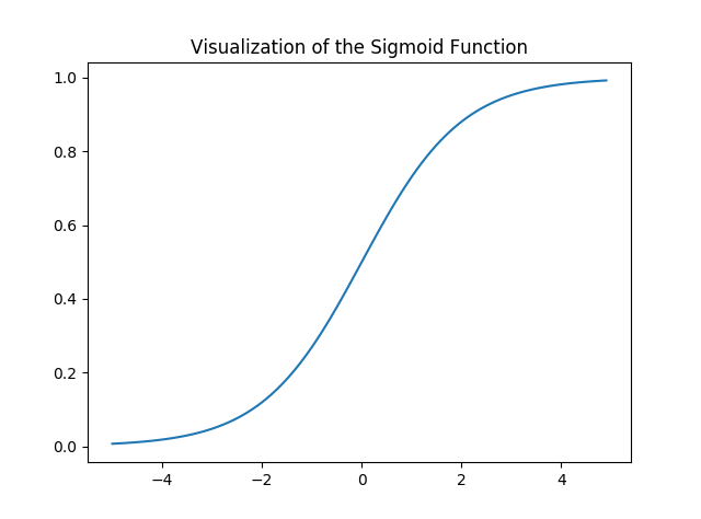
请注意,Sigmoid函数的范围是 (0, 1),这意味着结果值在 0 和 1 之间。Sigmoid函数的这一特性使其成为二进制分类激活函数的一个非常好的选择。同样for z = 0, Sigmoid(z) = 0.5 ,它是 Sigmoid函数范围的中点。
就像线性回归一样,我们需要找到成本函数J最小的w和b的最优值。在这种情况下,我们将使用由下式给出的 Sigmoid 交叉熵成本函数
然后将使用梯度下降优化此成本函数。
执行:
我们将从导入必要的库开始。我们将使用 Numpy 和 Tensorflow 进行计算,使用 Pandas 进行基本数据分析,使用 Matplotlib 进行绘图。我们还将使用Scikit-Learn的预处理模块对数据进行一次热编码。
# importing modules
import numpy as np
import pandas as pd
import tensorflow as tf
import matplotlib.pyplot as plt
from sklearn.preprocessing import OneHotEncoder
接下来我们将导入数据集。我们将使用著名的 Iris 数据集的一个子集。
data = pd.read_csv('dataset.csv', header = None)
print("Data Shape:", data.shape)

print(data.head())
输出:
Data Shape: (100, 4)
   0    1    2  3
0  0  5.1  3.5  1
1  1  4.9  3.0  1
2  2  4.7  3.2  1
3  3  4.6  3.1  1
4  4  5.0  3.6  1
现在让我们获取特征矩阵和相应的标签并进行可视化。
# Feature Matrix
x_orig = data.iloc[:, 1:-1].values

# Data labels
y_orig = data.iloc[:, -1:].values

print("Shape of Feature Matrix:", x_orig.shape)
print("Shape Label Vector:", y_orig.shape)
输出:
Shape of Feature Matrix: (100, 2)
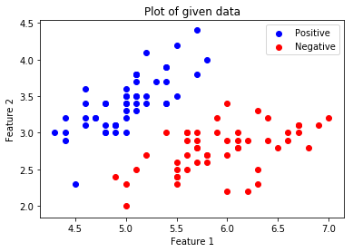
Shape Label Vector: (100, 1)可视化给定的数据。
# Positive Data Points
x_pos = np.array([x_orig[i] for i in range(len(x_orig))
                                    if y_orig[i] == 1])

# Negative Data Points
x_neg = np.array([x_orig[i] for i in range(len(x_orig))
                                    if y_orig[i] == 0])

# Plotting the Positive Data Points
plt.scatter(x_pos[:, 0], x_pos[:, 1], color = 'blue', label = 'Positive')

# Plotting the Negative Data Points
plt.scatter(x_neg[:, 0], x_neg[:, 1], color = 'red', label = 'Negative')

plt.xlabel('Feature 1')
plt.ylabel('Feature 2')
plt.title('Plot of given data')
plt.legend()

plt.show()
 .
.
现在我们将对数据进行 One Hot Encoding 以使其与算法一起使用。一种热编码将分类特征转换为更适合分类和回归算法的格式。我们还将设置学习率和时期数。
# Creating the One Hot Encoder
oneHot = OneHotEncoder()

# Encoding x_orig
oneHot.fit(x_orig)
x = oneHot.transform(x_orig).toarray()

# Encoding y_orig
oneHot.fit(y_orig)
y = oneHot.transform(y_orig).toarray()

alpha, epochs = 0.0035, 500
m, n = x.shape
print('m =', m)
print('n =', n)
print('Learning Rate =', alpha)
print('Number of Epochs =', epochs)
输出:
m = 100
n = 7
Learning Rate = 0.0035
Number of Epochs = 500现在我们将通过定义占位符X和Y开始创建模型,以便我们可以在训练过程中将训练示例x和y输入优化器。我们还将创建可通过梯度下降优化器优化的可训练变量W和b 。
# There are n columns in the feature matrix
# after One Hot Encoding.
X = tf.placeholder(tf.float32, [None, n])

# Since this is a binary classification problem,
# Y can take only 2 values.
Y = tf.placeholder(tf.float32, [None, 2])

# Trainable Variable Weights
W = tf.Variable(tf.zeros([n, 2]))

# Trainable Variable Bias
b = tf.Variable(tf.zeros([2]))
现在声明假设、成本函数、优化器和全局变量初始化器。
# Hypothesis
Y_hat = tf.nn.sigmoid(tf.add(tf.matmul(X, W), b))

# Sigmoid Cross Entropy Cost Function
cost = tf.nn.sigmoid_cross_entropy_with_logits(
                    logits = Y_hat, labels = Y)

# Gradient Descent Optimizer
optimizer = tf.train.GradientDescentOptimizer(
         learning_rate = alpha).minimize(cost)

# Global Variables Initializer
init = tf.global_variables_initializer()
在 Tensorflow 会话中开始训练过程。
# Starting the Tensorflow Session
with tf.Session() as sess:

    # Initializing the Variables
    sess.run(init)

    # Lists for storing the changing Cost and Accuracy in every Epoch
    cost_history, accuracy_history = [], []

    # Iterating through all the epochs
    for epoch in range(epochs):
        cost_per_epoch = 0

        # Running the Optimizer
        sess.run(optimizer, feed_dict = {X : x, Y : y})

        # Calculating cost on current Epoch
        c = sess.run(cost, feed_dict = {X : x, Y : y})

        # Calculating accuracy on current Epoch
        correct_prediction = tf.equal(tf.argmax(Y_hat, 1),
                                          tf.argmax(Y, 1))
        accuracy = tf.reduce_mean(tf.cast(correct_prediction,
                                                 tf.float32))

        # Storing Cost and Accuracy to the history
        cost_history.append(sum(sum(c)))
        accuracy_history.append(accuracy.eval({X : x, Y : y}) * 100)

        # Displaying result on current Epoch
        if epoch % 100 == 0 and epoch != 0:
            print("Epoch " + str(epoch) + " Cost: "
                            + str(cost_history[-1]))

    Weight = sess.run(W) # Optimized Weight
    Bias = sess.run(b)   # Optimized Bias

    # Final Accuracy
    correct_prediction = tf.equal(tf.argmax(Y_hat, 1),
                                      tf.argmax(Y, 1))
    accuracy = tf.reduce_mean(tf.cast(correct_prediction,
                                             tf.float32))
    print("\nAccuracy:", accuracy_history[-1], "%")
输出:
Epoch 100 Cost: 125.700202942
Epoch 200 Cost: 120.647117615
Epoch 300 Cost: 118.151592255
Epoch 400 Cost: 116.549999237

Accuracy: 91.0000026226 %
让我们绘制成本在各个时期的变化。
plt.plot(list(range(epochs)), cost_history)
plt.xlabel('Epochs')
plt.ylabel('Cost')
plt.title('Decrease in Cost with Epochs')

plt.show()

绘制各个时期的准确度变化。
plt.plot(list(range(epochs)), accuracy_history)
plt.xlabel('Epochs')
plt.ylabel('Accuracy')
plt.title('Increase in Accuracy with Epochs')

plt.show()

现在我们将为我们训练有素的分类器绘制决策边界。决策边界是将基础向量空间划分为两组的超曲面,每个组一组。
# Calculating the Decision Boundary
decision_boundary_x = np.array([np.min(x_orig[:, 0]),
                               np.max(x_orig[:, 0])])

decision_boundary_y = (- 1.0 / Weight[0]) *
      (decision_boundary_x * Weight + Bias)

decision_boundary_y = [sum(decision_boundary_y[:, 0]),
                       sum(decision_boundary_y[:, 1])]

# Positive Data Points
x_pos = np.array([x_orig[i] for i in range(len(x_orig))
                                    if y_orig[i] == 1])

# Negative Data Points
x_neg = np.array([x_orig[i] for i in range(len(x_orig))
                                    if y_orig[i] == 0])

# Plotting the Positive Data Points
plt.scatter(x_pos[:, 0], x_pos[:, 1],
  color = 'blue', label = 'Positive')

# Plotting the Negative Data Points
plt.scatter(x_neg[:, 0], x_neg[:, 1],
   color = 'red', label = 'Negative')

# Plotting the Decision Boundary
plt.plot(decision_boundary_x, decision_boundary_y)
plt.xlabel('Feature 1')
plt.ylabel('Feature 2')
plt.title('Plot of Decision Boundary')
plt.legend()

plt.show()
