具有 L 层的深度神经网络

本文旨在实现一个具有任意数量隐藏层的深度神经网络，每个隐藏层包含不同数量的神经元。我们将使用一些辅助函数来实现这个神经网络，最后，我们将结合这些函数来制作 L 层神经网络模型。
L——层深层神经网络结构（便于理解）

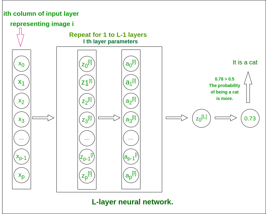
L——层神经网络

模型的结构是[LINEAR -> tanh](L-1 times) -> LINEAR -> SIGMOID。即，它有 L-1 层，使用双曲正切函数作为激活函数，然后是具有 sigmoid 激活函数的输出层。
更多关于激活函数
逐步实现神经网络：

Initialize the parameters for the L layers
Implement the forward propagation module
Compute the loss at the final layer
Implement the backward propagation module
Finally, update the parameters
Train the model using existing training dataset
Use trained parameters to test model

文章中遵循的命名约定以防止混淆：

• 网络中的每一层由一组两个参数W矩阵（权重矩阵）和b矩阵（偏置矩阵）表示。对于层， i这些参数分别表示为Wi和bi 。
• 层的线性输出 i 表示为Zi ，激活后的输出表示为Ai 。 Zi和Ai的尺寸相同。

权重和偏置矩阵的维度。
输入层的大小为 (x, m)，其中 m 是图像的数量。

Layer number	Shape of W	Shape of b	Linear Output	Shape of Activation
Layer 1	$(n[1], x)$	$(n[1], 1)$	$Z[1] = W[1]X + b[1]$	$(n[1], m)$
Layer 2	$(n[2], n[1])$	$(n[2], 1)$	$Z[2] = W[2]A[1] + b[2]$	$(n[2], m)$
:	$:$	$:$	$:$	$:$
Layer L – 1	$(n[L - 1], n[L - 2])$	$(n[L - 1], 1)$	$Z[L - 1] = W[L - 1]A[L - 2] + b[L - 1]$	$(n[L - 1], m)$
Layer L	$(n[L], n[L - 1])$	$(n[L], 1)$	$Z[L] = W[L]A[L - 1] + b[L]$	$(n[L], m)$

代码：导入所有必需的Python库。

Python3

import time
import numpy as np
import h5py
import matplotlib.pyplot as plt
import scipy
from PIL import Image
from scipy import ndimage

初始化：

• 我们将对权重矩阵使用随机初始化（以避免同一层中所有神经元的相同输出）。
• 偏差的零初始化。
• 每层中的神经元数量存储在 layer_dims 字典中，键为层号。

代码：

Python3

def initialize_parameters_deep(layer_dims):
    # 0th layer is the input layer with number
    # of columns stored in layer_dims.
    parameters = {}
 
    # number of layers in the network
    L = len(layer_dims)           
 
    for l in range(1, L):
        parameters['W' + str(l)] = np.random.randn(layer_dims[l],
                                        layer_dims[l - 1])*0.01
        parameters['b' + str(l)] = np.zeros((layer_dims[l], 1))
 
    return parameters

前向传播模块：
前向传播模块将分三步完成。我们将按此顺序完成三个功能：

• linear_forward（计算任何层的线性输出 Z）
• linear_activation_forward，其中激活将是 tanh 或 Sigmoid。
• L_model_forward [LINEAR -> tanh](L-1 次) -> LINEAR -> SIGMOID (整个模型)

线性前向模块（对所有示例进行矢量化）计算以下等式：
Zi = Wi * A(i – 1) + bi Ai = activation_func(Zi)
代码：

Python3

def linear_forward(A_prev, W, b):
 
    # cache is stored to be used in backward propagation module
    Z = np.dot(W, A_prev) + b
    cache = (A, W, b)
    return Z, cache

Python3

def sigmoid(Z):
 
    A = 1/(1 + np.exp(-Z))
    return A, {'Z' : Z}
 
def tanh(Z):
 
    A = np.tanh(Z)
    return A, {'Z' : Z}
 
def linear_activation_forward(A_prev, W, b, activation):
 
    # cache is stored to be used in backward propagation module
    if activation == "sigmoid":
        Z, linear_cache = linear_forward(A_prev, W, b)
        A, activation_cache = sigmoid(Z)
    elif activation == "tanh":
        Z, linear_cache = linear_forward(A_prev, W, b)
        A, activation_cache = tanh(Z)
    cache = (linear_cache, activation_cache)
 
    return A, cache

Python3

def L_model_forward(X, parameters):
    """
    Arguments:
    X -- data, numpy array of shape (input size, number of examples)
    parameters -- output of initialize_parameters_deep()
     
    Returns:
    AL -- last post-activation value
    caches -- list of caches containing:
                every cache of linear_activation_forward()
           (there are L-1 of them, indexed from 0 to L-1)
    """
 
    caches = []
    A = X
 
    # number of layers in the neural network
    L = len(parameters) // 2                 
     
    # Implement [LINEAR -> TANH]*(L-1). Add "cache" to the "caches" list.
    for l in range(1, L):
        A_prev = A
        A, cache = linear_activation_forward(A_prev,
                           parameters['W' + str(l)],
                   parameters['b' + str(l)], 'tanh')
 
        caches.append(cache)
     
    # Implement LINEAR -> SIGMOID. Add "cache" to the "caches" list.
    AL, cache = linear_activation_forward(A, parameters['W' + str(L)],
                                  parameters['b' + str(L)], 'sigmoid')
    caches.append(cache)
 
    return AL, caches

    $\[ {\Huge J = \frac{1}{m}\sum_{i=1}^{\m}y^{(i)}log(a^{[L][i]}) + (1 - y^{(i)})log(1 - a^{[L][i]})} \]$

我们将使用这个成本函数来测量所有训练数据的输出层的成本。
代码：

Python3

def compute_cost(AL, Y):
    """
    Implement the cost function defined by the equation.
    m = Y.shape[1]
    cost = (-1 / m)*(np.dot(np.log(AL), Y.T)+np.dot(np.log((1-AL)), (1 - Y).T))
 
    # To make sure your cost's shape is what we
    # expect (e.g. this turns [[20]] into 20).
    cost = np.squeeze(cost)     
 
    return cost

后向传播模块：
与前向传播模块类似，我们也将在该模块中实现三个功能。

• linear_backward（计算任何层的线性输出 Z）
• linear_activation_backward，其中激活将是 tanh 或 Sigmoid。
• L_model_backward [LINEAR -> tanh](L-1 次) -> LINEAR -> SIGMOID (整个模型反向传播)

对于第 i 层，线性部分为：Zi = Wi * A(i – 1) + bi
表示 dZi = $\frac{dJ}{dZi}$我们可以得到 dWi、dbi 和 dA(i – 1) 为 –
${\Huge dWi = \frac{dJ}{dWi} = \frac{1}{m}dZi * transpose(A(i - 1))}$
${\Huge dbi = \frac{dJ}{dbi} = \frac{1}{m}\sum_{i=1}^{\m}dZi}$
${\Huge dA(i - 1) = \frac{dJ}{dA(i - 1)} = transpose(Wi)*dZi }$
这些方程是使用微积分制定的，并使用 np.dot()函数保持矩阵的维数适合于矩阵点乘法。
代码：用于实现的Python代码

Python3

def linear_backward(dZ, cache):
 
    A_prev, W, b = cache
    m = A_prev.shape[1]
    dW = (1 / m)*np.dot(dZ, A_prev.T)
    db = (1 / m)*np.sum(dZ, axis = 1, keepdims = True)
    dA_prev = np.dot(W.T, dZ)
     
    return dA_prev, dW, db

在这里，我们将计算 sigmoid 和 tanh 函数的导数。了解激活函数的推导
代码：

Python3

def sigmoid_backward(dA, activation_cache):
 
    Z = activation_cache['Z']
    A = sigmoid(Z)
    return dA * (A*(1 - A))    # A*(1 - A) is the derivative of sigmoid function
 
def tanh_backward(dA, activation_cache):
 
    Z = activation_cache['Z']
    A = sigmoid(Z)
    return dA * (1 -np.power(A, 2))  
    # A*(1 -

L-model-backward：
回想一下，当您实现 L_model_forward函数时，在每次迭代中，您都存储了一个包含（X、W、b 和 Z）的缓存。在反向传播模块中，您将使用这些变量来计算梯度。

Python3

def L_model_backward(AL, Y, caches):
    """
    AL -- probability vector, output of the forward propagation (L_model_forward())
    Y -- true "label" vector (containing 0 if non-cat, 1 if cat)
    caches -- list of caches containing:
                every cache of linear_activation_forward() with "tanh"
                (it's caches[l], for l in range(L-1) i.e l = 0...L-2)
                the cache of linear_activation_forward() with "sigmoid"
                 (it's caches[L-1])
     
    Returns:
    grads -- A dictionary with the gradients
             grads["dA" + str(l)] = ...
             grads["dW" + str(l)] = ...
             grads["db" + str(l)] = ...
    """
    grads = {}
    L = len(caches) # the number of layers
    m = AL.shape[1]
    Y = Y.reshape(AL.shape) # after this line, Y is the same shape as AL
     
    # Initializing the backpropagation
    # derivative of cost with respect to AL
  
    dAL = - (np.divide(Y, AL) - np.divide(1 - Y, 1 - AL))
     
    # Lth layer (SIGMOID -> LINEAR) gradients. Inputs: "dAL, current_cache".
    # Outputs: "grads["dAL-1"], grads["dWL"], grads["dbL"]
    current_cache = caches[L - 1]
    grads["dA" + str(L-1)], grads["dW" + str(L)], grads["db" + str(L)] = \
                  linear_activation_backward(dAL, current_cache, 'sigmoid')
     
    # Loop from l = L-2 to l = 0
    for l in reversed(range(L-1)):
        current_cache = caches[l]
        dA_prev_temp, dW_temp, db_temp = linear_activation_backward(
                    grads['dA' + str(l + 1)], current_cache, 'tanh')
        grads["dA" + str(l)] = dA_prev_temp
        grads["dW" + str(l + 1)] = dW_temp
        grads["db" + str(l + 1)] = db_temp
 
    return grads

更新参数：
Wi = Wi – a*dWi
bi = bi – a*dbi
（其中 a 是一个适当的常数，称为学习率）

Python3

def update_parameters(parameters, grads, learning_rate):
    L = len(parameters) // 2 # number of layers in the neural network
 
    # Update rule for each parameter. Use a for loop.
    for l in range(L):
        parameters["W" + str(l + 1)] = parameters["W" + str(l + 1)] - learning_rate * grads['dW' + str(l + 1)]
        parameters["b" + str(l + 1)] = parameters['b' + str(l + 1)] - learning_rate * grads['db' + str(l + 1)]
 
    return parameters

代码：训练模型
现在是时候将之前编写的所有函数累加起来，形成最终的 L 层神经网络模型了。 L_layer_model 中的参数 X 将是训练数据集，Y 是相应的标签。

Python3

def L_layer_model(X, Y, layers_dims, learning_rate = 0.0075, num_iterations = 3000, print_cost = False):
    """
    Arguments:
    X -- data, numpy array of shape (num_px * num_px * 3, number of examples)
    Y -- true "label" vector (containing 0 if cat, 1 if non-cat),
                                 of shape (1, number of examples)
    layers_dims -- list containing the input size and each layer size,
                                      of length (number of layers + 1).
    learning_rate -- learning rate of the gradient descent update rule
    num_iterations -- number of iterations of the optimization loop
    print_cost -- if True, it prints the cost every 100 steps
     
    Returns:
    parameters -- parameters learned by the model. They can then be used to predict.
    """
 
    np.random.seed(1)
    costs = []                         # keep track of cost
 
    parameters = initialize_parameters_deep(layers_dims)
     
    # Loop (gradient descent)
    for i in range(0, num_iterations):
 
        # Forward propagation: [LINEAR -> TANH]*(L-1) -> LINEAR -> SIGMOID.
        AL, caches = L_model_forward(X, parameters)
 
        # Compute cost.
        cost = compute_cost(AL, Y)
     
        # Backward propagation.
        grads = L_model_backward(AL, Y, caches)
 
        # Update parameters.
        parameters = update_parameters(parameters, grads, learning_rate)
                 
        # Print the cost every 100 training example
        if print_cost and i % 100 == 0:
            print ("Cost after iteration % i: % f" %(i, cost))
        if print_cost and i % 100 == 0:
            costs.append(cost)
             
    # plot the cost
    plt.plot(np.squeeze(costs))
    plt.ylabel('cost')
    plt.xlabel('iterations (per hundreds)')
    plt.title("Learning rate =" + str(learning_rate))
    plt.show()
     
    return parameters

代码：实现预测函数以测试提供的图像。

Python3

def predict(parameters, path_image):
 
    my_image = path_image
    image = np.array(ndimage.imread(my_image, flatten = False))
    my_image = scipy.misc.imresize(image,
                  size =(num_px, num_px)).reshape((
                          num_px * num_px * 3, 1))
 
    my_image = my_image / 255.
    output, cache = L_model_forward(my_image, parameters)
    output = np.squeeze(output)
    prediction = round(output)
    if(prediction == 1):
        label = "Cat picture"
    else:
        label = "Non-Cat picture"   # If the model is trained to recognize a cat image.
    print ("y = " + str(prediction) + ", your L-layer model predicts a \"" + label)

提供 layers_dims = [12288, 20, 7, 5, 1] 当这个模型用适当数量的训练数据集训练时，它在测试数据上的准确率高达80% 。
在使用适当数量的训练数据集进行训练后找到参数。

Python3

{'W1': array([[ 0.01672799, -0.00641608, -0.00338875, ..., -0.00685887,
        -0.00593783,  0.01060475],
       [ 0.01395808,  0.00407498, -0.0049068, ...,  0.01317046,
         0.00221326,  0.00930175],
       [-0.00123843, -0.00597204,  0.00472214, ...,  0.00101904,
        -0.00862638, -0.00505112],
       ...,
       [ 0.00140823, -0.00137711,  0.0163992, ..., -0.00846451,
        -0.00761603, -0.00149162],
       [-0.00168698, -0.00618577, -0.01023935, ...,  0.02050705,
        -0.00428185,  0.00149319],
       [-0.01770891, -0.0067836,  0.00756873, ...,  0.01730701,
         0.01297081, -0.00322241]]), 'b1': array([[  3.85542520e-03],
       [  8.18087056e-03],
       [  6.52138546e-03],
       [  2.85633678e-03],
       [  6.01081275e-03],
       [  8.17122684e-04],
       [  3.72986493e-04],
       [  7.05992009e-04],
       [  4.36344692e-04],
       [  1.90827285e-03],
       [ -6.51686461e-03],
       [  6.97258125e-03],
       [ -1.08988113e-03],
       [  5.40858776e-03],
       [  8.16752511e-03],
       [ -1.05298871e-02],
       [ -9.05267219e-05],
       [ -5.13240993e-04],
       [  1.42355924e-03],
       [ -2.40912130e-03]]), 'W2': array([[  2.02109232e-01,  -3.08645240e-01,  -3.77620591e-01,
         -4.02563039e-02,   5.90753267e-02,   1.23345558e-01,
          3.08047246e-01,   4.71201576e-02,   5.29892230e-02,
          1.34732883e-01,   2.15804697e-01,  -6.34295948e-01,
         -1.56081006e-01,   1.01905466e-01,  -1.50584386e-01,
          5.31219819e-02,   1.14257132e-01,   4.20697960e-01,
          1.08551174e-01,  -2.18735332e-01],
       [  3.57091131e-01,  -1.40997155e-01,   3.70857247e-01,
          2.53207014e-01,  -1.12596978e-01,  -3.15179195e-01,
         -2.48100731e-01,   4.72723584e-01,  -7.71870940e-02,
          5.39834663e-01,  -1.17927181e-02,   6.45463019e-02,
          2.73704423e-02,   4.30157714e-01,   1.59318390e-01,
         -6.48089126e-01,  -1.71894333e-01,   1.77933527e-01,
          1.54736463e-01,  -7.26815274e-02],
       [  2.96501527e-01,   2.43056424e-01,  -1.22400000e-02,
          2.69275366e-02,   3.76041647e-01,  -1.70245407e-01,
         -2.95343754e-02,  -7.35716150e-02,  -1.80179693e-01,
         -5.77515859e-03,  -6.38323383e-01,   6.94950669e-02,
          7.66137263e-02,   3.66599261e-01,   5.40904716e-02,
         -1.51814996e-01,  -2.61672559e-01,   1.35946854e-01,
          4.21086332e-01,  -2.71073484e-01],
       [  1.42186042e-01,  -2.66789439e-01,   4.57188131e-01,
          2.84732743e-02,  -5.49143391e-02,  -3.96786581e-02,
         -1.68668726e-01,  -1.46525541e-01,   3.25325993e-03,
         -1.13045329e-01,   4.03935681e-01,  -3.92214264e-01,
          5.25325051e-04,  -3.69642647e-01,  -1.15812921e-01,
          1.32695899e-01,   3.20810624e-01,   1.88127350e-01,
         -4.82784806e-02,  -1.48816756e-01],
       [ -1.65469406e-01,   4.24741323e-01,  -5.76900900e-01,
          1.58084434e-01,  -2.90965849e-01,   3.40124014e-02,
         -2.62189635e-01,   2.66917709e-01,   4.77530579e-01,
         -1.73491365e-01,  -1.48434710e-01,  -6.91270097e-02,
          5.42923817e-03,  -2.85173244e-01,   6.40701002e-02,
         -7.33126171e-02,   1.43543481e-01,   7.82250247e-02,
         -1.47535352e-01,  -3.99073661e-01],
       [ -2.05468389e-01,   1.66914752e-01,   2.15918881e-01,
          2.21774761e-01,   2.52527888e-01,   2.64464223e-01,
         -3.07796263e-02,  -3.06999665e-01,   3.45835418e-01,
          1.05973413e-01,  -3.47687682e-01,   9.13383273e-02,
          3.97150339e-02,  -3.14285982e-01,   2.22363710e-01,
         -3.93921988e-01,  -9.70224337e-02,  -3.03701358e-01,
          1.40075127e-01,  -4.56621577e-01],
       [  2.06819296e-01,  -2.39537245e-01,  -4.06133490e-01,
          5.92692802e-02,   8.95374287e-02,  -3.27700300e-01,
         -6.89856027e-02,  -6.13447906e-01,   1.89927573e-01,
         -1.42814095e-01,   1.77958823e-03,  -1.34407806e-01,
          9.34036862e-02,  -2.00549616e-02,   9.01789763e-02,
          3.81627943e-01,   3.30416268e-01,  -1.76566228e-02,
          9.28388267e-02,  -1.16167106e-01]]), 'b2': array([[-0.00088887],
       [ 0.02357712],
       [ 0.01858614],
       [-0.00567557],
       [ 0.00636179],
       [ 0.02362429],
       [-0.00173074]]), 'W3': array([[ 0.20939786,  0.21977478,  0.77135171, -1.07520777, -0.64307173,
        -0.24097649, -0.15626735],
       [-0.57997618,  0.30851841, -0.03802324, -0.13489975,  0.23488207,
         0.76248961, -0.34515092],
       [ 0.15990295,  0.5163969,  0.15284381,  0.42790606, -0.05980168,
         0.87865156, -0.01031899],
       [ 0.52908282,  0.93882471,  1.23044256, -0.01481286,  0.41024244,
         0.18731983, -0.01414658],
       [-0.96753783, -0.30492002,  0.54060558, -0.18776932, -0.39245146,
         0.20654634, -0.58863038]]), 'b3': array([[ 0.8623361 ],
       [-0.00826002],
       [-0.01151116],
       [-0.06844291],
       [-0.00833715]]), 'W4': array([[-0.83045967,  0.18418824,  0.85885352,  1.41024115,  0.12713131]]), 'b4': array([[-1.73123633]])}

测试自定义图像

Python3

my_image = "https://www.pexels.com / photo / adorable-animal-blur-cat-617278/"
predict(parameters, my_image)

带有学习参数的输出：

y = 1, your L-layer model predicts a Cat picture.