从头开始具有正向和反向传播的深度神经网络 - Python

本文旨在从头开始实现一个深度神经网络。我们将实现一个包含一个隐藏层的深度神经网络，该隐藏层具有四个单元和一个输出层。实施将从头开始，并将实施以下步骤。
算法：

1. Visualizing the input data
2. Deciding the shapes of Weight and bias matrix
3. Initializing matrix, function to be used
4. Implementing the forward propagation method
5. Implementing the cost calculation
6. Backpropagation and optimizing
7. prediction and visualizing the output

模型架构：
该模型的架构由下图定义，其中隐藏层使用双曲正切作为激活函数，而输出层（即分类问题）使用 sigmoid函数。

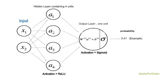
模型架构

权重和偏差：
将用于两个层的权重和偏差必须首先声明，并且其中的权重将随机声明以避免所有单元的相同输出，而偏差将初始化为零。计算将从头开始并根据下面给出的规则进行，其中 W1、W2 和 b1、b2 分别是第一层和第二层的权重和偏差。这里 A 代表特定层的激活。

$\begin{array}{c} z^{[1]}=W^{[1]} x+b^{[1]} \\ a^{[1](i)}=\tanh \left(z^{[1]}\right) \\ z^{[2]}=W^{[2]} a^{[1]}+b^{[2]} \\ \hat{y}=a^{[2]}=\sigma\left(z^{[2]}\right) \\ y_{\text {prediction}}=\left\{\begin{array}{ll} 1 & \text { if } a^{[2]}>0.5 \\ 0 & \text { otherwise } \end{array}\right. \end{array}$
成本函数：
上述模型的成本函数将与逻辑回归使用的成本函数有关。因此，在本教程中，我们将使用成本函数：

$L = Y * \log \left(Y_{-} p r e d\right)+(1-Y) * \log \left(1-Y_{-} p r e d\right)$

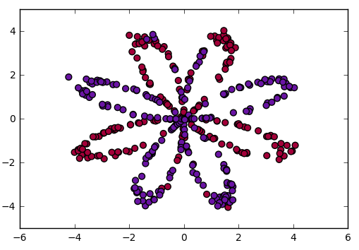
代码：可视化数据

# Package imports
import numpy as np
import matplotlib.pyplot as plt
# here planar_utils.py can be found on its github repo
from planar_utils import plot_decision_boundary, sigmoid, load_planar_dataset
# Loading the Sample data
X, Y = load_planar_dataset()
  
# Visualize the data:
plt.scatter(X[0, :], X[1, :], c = Y, s = 40, cmap = plt.cm.Spectral);

代码：初始化权重和偏差矩阵
这里隐藏单元的数量是 4，因此，W1 权重矩阵的形状为 (4, 特征数)，偏置矩阵的形状为 (4, 1)，广播后将根据权重矩阵相加对上式。同样可以应用于W2。

# X --> input dataset of shape (input size, number of examples)
# Y --> labels of shape (output size, number of examples)
  
W1 = np.random.randn(4, X.shape[0]) * 0.01
b1 = np.zeros(shape =(4, 1))
  
W2 = np.random.randn(Y.shape[0], 4) * 0.01
b2 = np.zeros(shape =(Y.shape[0], 1))

代码：前向传播：
现在我们将使用 W1、W2 和偏置 b1、b2 执行前向传播。在这一步中，相应的输出在定义为 forward_prop 的函数中计算。

def forward_prop(X, W1, W2, b1, b2):
  
    Z1 = np.dot(W1, X) + b1
    A1 = np.tanh(Z1)
    Z2 = np.dot(W2, A1) + b2
    A2 = sigmoid(Z2)
      
    # here the cache is the data of previous iteration
    # This will be used for backpropagation
    cache = {"Z1": Z1,
             "A1": A1,
             "Z2": Z2,
             "A2": A2}
      
    return A2, cache

代码：定义成本函数：

# Here Y is actual output
def compute_cost(A2, Y):
    m = Y.shape[1]
    # implementing the above formula
    cost_sum = np.multiply(np.log(A2), Y) + np.multiply((1 - Y), np.log(1 - A2))
    cost = - np.sum(logprobs) / m
      
    # Squeezing to avoid unnecessary dimensions
    cost = np.squeeze(cost)
    return cost

代码：最后反向传播函数：
这是一个非常关键的步骤，因为它涉及大量线性代数来实现深度神经网络的反向传播。求导数的公式可以用线性代数的一些数学概念推导出来，这里我们不打算推导。请记住，dZ、dW、db 是成本函数wrt 加权和、权重、层偏差的导数。

def back_propagate(W1, b1, W2, b2, cache):
   
    # Retrieve also A1 and A2 from dictionary "cache"
    A1 = cache['A1']
    A2 = cache['A2']
  
    # Backward propagation: calculate dW1, db1, dW2, db2. 
    dZ2 = A2 - Y
    dW2 = (1 / m) * np.dot(dZ2, A1.T)
    db2 = (1 / m) * np.sum(dZ2, axis = 1, keepdims = True)
  
    dZ1 = np.multiply(np.dot(W2.T, dZ2), 1 - np.power(A1, 2))
    dW1 = (1 / m) * np.dot(dZ1, X.T)
    db1 = (1 / m) * np.sum(dZ1, axis = 1, keepdims = True)
      
    # Updating the parameters according to algorithm
    W1 = W1 - learning_rate * dW1
    b1 = b1 - learning_rate * db1
    W2 = W2 - learning_rate * dW2
    b2 = b2 - learning_rate * db2
  
    return W1, W2, b1, b2

代码：训练自定义模型现在我们将使用上面定义的函数来训练模型，可以根据处理单元的便利性和能力来放置时期。

# Please note that the weights and bias are global 
# Here num_iteration is epochs
for i in range(0, num_iterations):
    
        # Forward propagation. Inputs: "X, parameters". return: "A2, cache".
        A2, cache = forward_propagation(X, W1, W2, b1, b2)
          
        # Cost function. Inputs: "A2, Y". Outputs: "cost".
        cost = compute_cost(A2, Y)
   
        # Backpropagation. Inputs: "parameters, cache, X, Y". Outputs: "grads".
        W1, W2, b1, b2 = backward_propagation(W1, b1, W2, b2, cache)
          
        # Print the cost every 1000 iterations
        if print_cost and i % 1000 == 0:
            print ("Cost after iteration % i: % f" % (i, cost))

带有学习参数的输出
训练模型后，使用上面的 forward_propagate函数获取权重并预测结果，然后使用这些值绘制输出图。您将获得类似的输出。

可视化数据边界

结论：
深度学习是一个掌握基础知识的人夺取宝座的世界，因此，请尝试开发如此强大的基础知识，以便之后您可能成为可能会彻底改变社区的新模型架构的开发者。