Python – 使用 Iris 数据集的 Pandas 基础

Python语言是最流行的编程语言之一，因为它比其他语言更动态。 Python是一种用于通用编程的简单高级和开源语言。它有许多开源库，Pandas 就是其中之一。 Pandas 是一个强大、快速、灵活的开源库，用于数据分析和数据帧/数据集的操作。 Pandas 可用于在不同格式的数据集中读取和写入数据，例如 CSV（逗号分隔值）、txt、xls（Microsoft Excel）等。
在这篇文章中，您将了解Python中 Pandas 的各种功能以及如何使用它来练习。
先决条件：有关Python编码的基本知识。
安装：
所以如果你是刚开始练习 Pandas，那么首先你应该在你的系统上安装 Pandas。
转到命令提示符并以管理员身份运行它。确保您已连接到 Internet 以将其下载并安装到您的系统上。
然后输入“ pip install pandas ”，然后按回车键。

从这里下载数据集“Iris.csv”
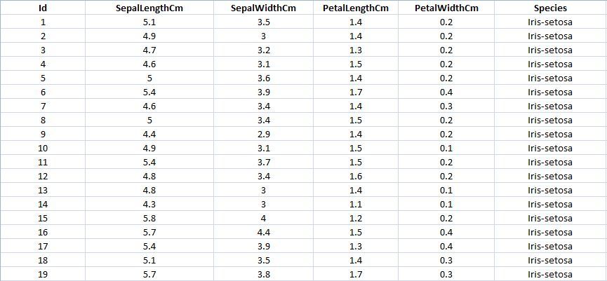
Iris 数据集是数据科学的 Hello World，因此，如果您的职业生涯开始于数据科学和机器学习，您将在这个著名的数据集上练习基本的 ML 算法。鸢尾花数据集包含花瓣长度、花瓣宽度、萼片长度、萼片宽度和物种类型等五列。
鸢尾是一种开花植物，研究人员测量了不同鸢尾花的各种特征并进行了数字记录。

熊猫入门：
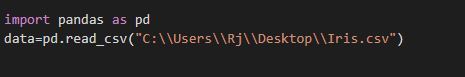
代码：导入 pandas 以在我们的代码中作为 pd 使用。

Python3

import pandas as pd

代码：读取数据集“Iris.csv”。

Python3

data = pd.read_csv("your downloaded dataset location ")

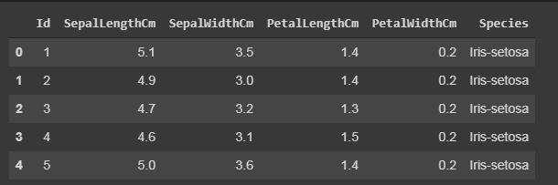
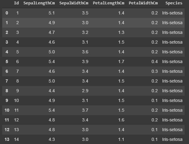
代码：显示数据集的顶行及其列
函数head() 将显示数据集的前 5 行，该函数的默认值为 5，即不给它参数时将显示前 5 行。

Python3

data.head()

输出：

随机显示行数。
在 sample()函数中，它也会根据给定的参数显示行，但它会随机显示行。

Python3

data.sample(10)

输出：

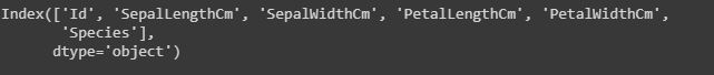
代码：显示列数和列名。
column()函数以列表形式打印数据集的所有列。

Python3

data.columns

输出：

代码：显示数据集的形状。
数据集的形状意味着打印该特定数据集的总行数或条目数以及列数或特征的总数。

Python3

#The first one is the number of rows and
# the other one is the number of columns.
data.shape

输出：

代码：显示整个数据集

Python3

print(data)

输出：

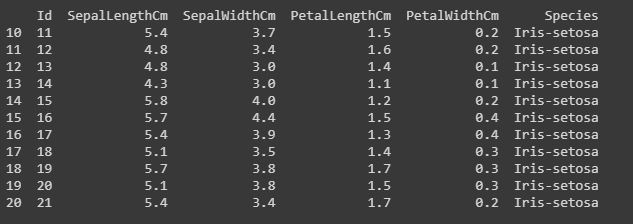
代码：切片行。
切片意味着如果要打印或处理从第 10 行到第 20 行的特定行组。

Python3

#data[start:end]
#start is inclusive whereas end is exclusive
print(data[10:21])
# it will print the rows from 10 to 20.
 
# you can also save it in a variable for further use in analysis
sliced_data=data[10:21]
print(sliced_data)

输出：

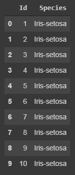
代码：仅显示特定列。
在任何数据集中，有时只需要处理特定的特征或列，因此我们可以通过以下代码来完成。

Python3

#here in the case of Iris dataset
#we will save it in a another variable named "specific_data"
 
specific_data=data[["Id","Species"]]
#data[["column_name1","column_name2","column_name3"]]
 
#now we will print the first 10 columns of the specific_data dataframe.
print(specific_data.head(10))

输出：

过滤：使用“iloc”和“loc”函数显示特定的行。

“loc”函数使用行的索引名称来显示数据集的特定行。
“iloc”函数使用行的索引整数，它提供有关行的完整信息。
代码：

Python3

#here we will use iloc
 
data.iloc[5]
#it will display records only with species "Iris-setosa".
data.loc[data["Species"] == "Iris-setosa"]

输出：

iloc()[/标题]

定位（）

代码：使用“value_counts()”计算唯一值的计数。
value_counts()函数计算特定实例或数据发生的次数。

Python3

#In this dataset we will work on the Species column, it will count number of times a particular species has occurred.
data["Species"].value_counts()
#it will display in descending order.

输出：

计算特定列的总和、平均值和众数。
我们还可以计算任何整数列的总和、均值和众数，就像我在下面的代码中所做的那样。

Python3

# data["column_name"].sum()
 
sum_data = data["SepalLengthCm"].sum()
mean_data = data["SepalLengthCm"].mean()
median_data = data["SepalLengthCm"].median()
 
print("Sum:",sum_data, "\nMean:", mean_data, "\nMedian:",median_data)

输出：

代码：从列中提取最小值和最大值。
从特定列或行中识别最小和最大整数也可以在数据集中完成。

Python3

min_data=data["SepalLengthCm"].min()
max_data=data["SepalLengthCm"].max()
 
print("Minimum:",min_data, "\nMaximum:", max_data)

输出：

代码：向数据集添加列。
如果想在我们的数据集中添加一个新列，因为我们正在进行任何计算或从数据集中提取一些信息，并且如果您想将其保存为一个新列。这可以通过以下代码来完成，方法是我们添加了所有列的所有整数值。

Python3

# For example, if we want to add a column let say "total_values",
# that means if you want to add all the integer value of that particular
# row and get total answer in the new column "total_values".
# first we will extract the columns which have integer values.
cols = data.columns
 
# it will print the list of column names.
print(cols)
 
# we will take that columns which have integer values.
cols = cols[1:5]
 
# we will save it in the new dataframe variable
data1 = data[cols]
 
# now adding new column "total_values" to dataframe data.
data["total_values"]=data1[cols].sum(axis=1)
 
# here axis=1 means you are working in rows,
# whereas axis=0 means you are working in columns.

输出：

代码：重命名列。
在Python pandas 库中也可以重命名我们的列名。我们使用了 rename()函数，我们在其中创建了一个字典“newcols”来更新我们的新列名。下面的代码说明了这一点。

Python3

newcols={
"Id":"id",
"SepalLengthCm":"sepallength"
"SepalWidthCm":"sepalwidth"}
 
data.rename(columns=newcols,inplace=True)
 
print(data.head())

输出：

格式和样式：
可以使用 Dataframe.style函数将条件格式应用于您的数据框。样式用于可视化您的数据，可视化数据集的最便捷方式是表格形式。
在这里，我们将突出显示每行和每列的最小值和最大值。

Python3

#this is an example of rendering a datagram,
which is not visualised by any styles.
data.style

输出：

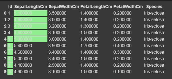
现在我们将使用 Styler.apply函数突出显示最大和最小列、行和整个数据框。 Styler.apply函数根据关键字参数轴传递数据帧的每一列或每一行。对于按列使用axis = 0，按行使用axis = 1，对于整个表格一次使用axis = None。

Python3

# we will here print only the top 10 rows of the dataset,
# if you want to see the result of the whole dataset remove
#.head(10) from the below code
 
data.head(10).style.highlight_max(color='lightgreen', axis=0)
 
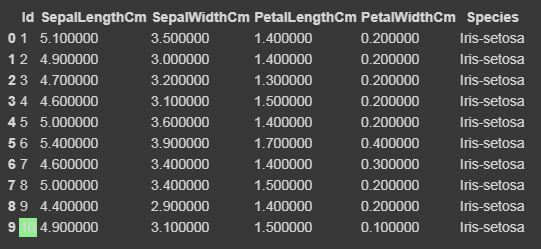
data.head(10).style.highlight_max(color='lightgreen', axis=1)
 
data.head(10).style.highlight_max(color='lightgreen', axis=None)

输出：

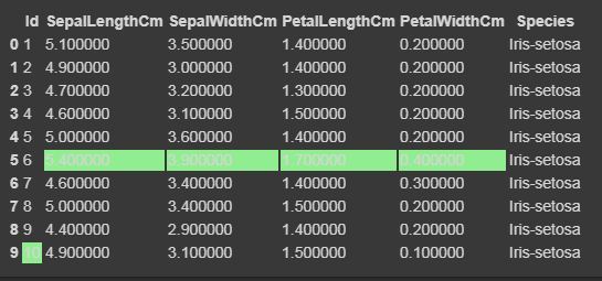
轴=0

轴=1

对于轴=无

代码：清理和检测缺失值
在这个数据集中，我们现在将尝试找到缺失值，即 NaN，这可能由于多种原因而发生。

Python3

data.isnull()
#if there is data is missing, it will display True else False.

输出：

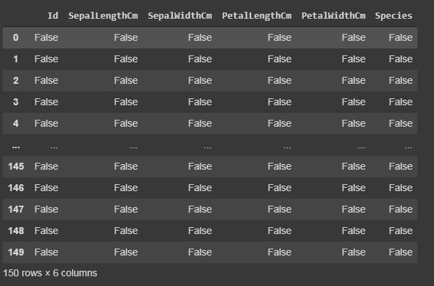
一片空白（）

代码：总结缺失值。
我们将显示每列中存在多少缺失值。

Python3

data.isnull.sum()

输出：

热图：导入 seaborn
热图是一种数据可视化技术，用于将数据集分析为二维颜色。基本上，它显示了数据集中所有数值变量之间的相关性。热图是 Seaborn 库的一个属性。
代码：

Python3

import seaborn as sns
 
iris = sns.load_dataset("iris")
sns.heatmap(iris.corr(),camp = "YlGnBu", linecolor = 'white', linewidths = 1)

输出：

代码：使用整数格式用数值注释每个单元格

Python3

sns.heatmap(iris.corr(),camp = "YlGnBu", linecolor = 'white', linewidths = 1, annot = True )

输出：

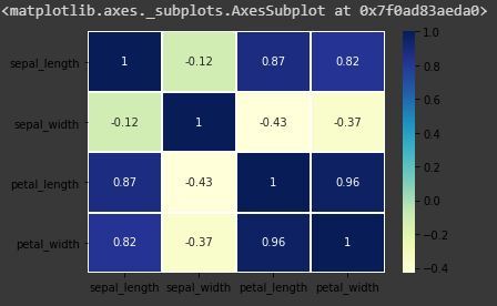
annot=True 的热图

熊猫数据框相关性：
Pandas 相关性用于确定数据集所有列的成对相关性。在 dataframe.corr() 中，缺失值被排除，非数字列也被忽略。
代码：

Python3

data.corr(method='pearson')

输出：

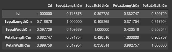
数据.corr()

输出数据框可以看作是对于任何单元格，行变量与列变量的相关性就是该单元格的值。变量与其自身的相关性为 1。因此，所有对角线值均为 1.00。
多元分析：
配对图用于可视化每种类型的列变量之间的关系。仅通过一行代码实现，代码如下：
代码：

Python3

g = sns.pairplot(data,hue="Species")

输出：

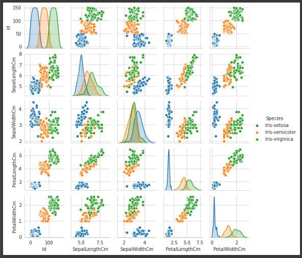
变量“物种”的配对图，使其更易于理解。