在 R 中使用 ggplot2 可视化相关矩阵

在本文中，我们将讨论如何使用 R 编程语言中的 ggplot2 包来可视化相关矩阵。

为此，我们将安装一个名为ggcorrplot包的包。在这个包的帮助下，我们可以轻松地可视化相关矩阵。我们还可以使用此包中存在的函数来计算相关 p 值的矩阵。 corr_pmat()用于计算 p 值的相关矩阵， ggcorrplot()用于使用 ggplot 显示相关矩阵。

句法 ：

corr_pmat(x,..)

其中 x 是数据框或矩阵

句法：

ggcorrplot(corr, method = c(“circle”, “square”), type = c(“full”, “lower”, “upper”), title = “”, ggtheme=ggplot2::theme_minimal, show.legend = TRUE, legend.title = “corr”, show.diag = FALSE, colors = c(“blue”, “white”, “red”), outline.color = “gray”, hc.order = FALSE, hc.method = “complete”, lab = FALSE, lab_col =”black”, p.mat = NULL,.. )

入门

我们将首先使用install.packages()安装和library()加载包来安装和加载ggcorrplot和ggplot2包。我们需要一个数据集来构建我们的相关矩阵，然后将其可视化。我们将在cor()函数的帮助下创建我们的相关矩阵，该函数计算相关系数。计算相关矩阵后，我们将使用corr_pmat()函数计算相关 p 值的矩阵。接下来，我们将使用 ggplot2 在ggcorrplot()函数的帮助下可视化相关矩阵。

创建相关矩阵

我们将采用一个示例数据集来更好地解释我们的方法。我们将采用内置的 USArrests 数据集，并按照上述方法可视化其相关矩阵。我们将使用 data()函数读取数据，并在 cor()函数的帮助下创建相关矩阵以计算相关系数。 round()函数用于将值四舍五入为特定的十进制值。我们将使用 cor_pmat()函数来计算具有 p 值的相关矩阵。

Syntax : 

correlation_matrix <- round(cor(data),1)

Parameters : 

• correlation_matrix : Variable for correlation matrix used to visualize.
• data : data is our dataset which we have taken for visualization. 

Syntax:

corrp.mat <- cor_pmat(data)

Parameters :

• corrp.mat : Variable for correlation matrix with p-values.
• data : It is our dataset taken for creating correlation matrix with p-values.

示例：创建相关矩阵

R

# Installing and loading the ggcorrplot package
install.packages("ggcorrplot")
library(ggcorrplot)
  
# Reading the data
data(USArrests)
  
# Computing correlation matrix
correlation_matrix <- round(cor(USArrests),1)
  
head(correlation_matrix[, 1:4])
  
# Computing correlation matrix with p-values
corrp.mat <- cor_pmat(USArrests)
  
head(corrp.mat[, 1:4])

输出 ：

可视化相关矩阵

现在因为我们有一个相关矩阵和带有 p 值的相关矩阵，我们现在将尝试可视化这个相关矩阵。第一个可视化是使用 ggcorrplot()函数并以正方形和圆形方法的形式绘制我们的相关矩阵。

Syntax :

ggcorrplot(correlation_matrix, method= c(“circle”,”square”))

Parameters : 

• correlation_matrix : The correlation matrix for visualization.
• method : It is a character value used for visualization methods.

示例：使用不同方法可视化相关矩阵

电阻

library(ggplot2)
library(ggcorrplot)
  
# Reading the data
data(USArrests)
  
# Computing correlation matrix
correlation_matrix <- round(cor(USArrests),1)
  
# Computing correlation matrix with p-values
corrp.mat <- cor_pmat(USArrests)
  
# Visualizing the correlation matrix using 
# square and circle methods
ggcorrplot(correlation_matrix, method ="square")
ggcorrplot(correlation_matrix, method ="circle")

输出 ：

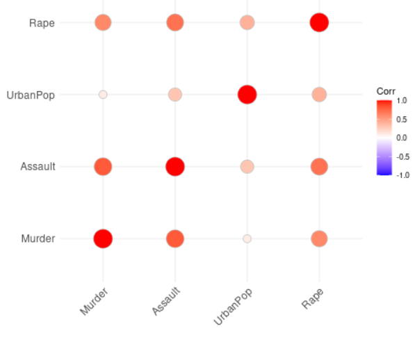
使用循环法的相关矩阵

平方法相关矩阵

使用不同的布局可视化相关矩阵

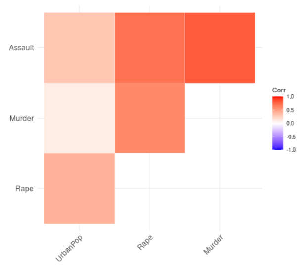
• 接下来，我们将在我们的相关矩阵中可视化相关图布局类型，并在 ggcorrplot()函数提供 hc.order 和 type 作为下三角布局的下限和上三角布局的上限作为参数。

Syntax : ggcorrplot(correlation_matrix, hc.order = TRUE, type = c(“upper”, “lower”), outline.color = “white”)

Parameters :

• correlation_matrix : The correlation matrix used for visualization.
• hc.order : If it is true, then the correlation matrix will be ordered.
• type : It is the arrangement of the character to display.
• outline.color : It is the outline color of the square or circle.

示例：使用不同布局可视化相关矩阵

电阻

library(ggplot2)
library(ggcorrplot)
  
# Reading the data
data(USArrests)
  
# Computing correlation matrix
correlation_matrix <- round(cor(USArrests),1)
  
# Computing correlation matrix with p-values
corrp.mat <- cor_pmat(USArrests)
  
# Visualizing upper and lower triangle layouts
ggcorrplot(correlation_matrix, hc.order =TRUE, type ="lower", 
           outline.color ="white")
  
ggcorrplot(correlation_matrix, hc.order =TRUE, type ="upper", 
           outline.color ="white")

输出 ：

上层布局的相关矩阵

具有较低布局的相关矩阵

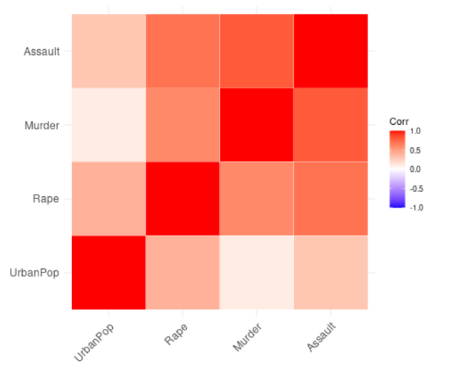
重新排序相关矩阵

我们现在将通过使用层次聚类对矩阵重新排序来可视化我们的相关矩阵。我们将使用 ggcorrplot函数和相关矩阵、hc.order、outline.color 作为参数来做到这一点。

Syntax : 

ggcorrplot(correlation_matrix, hc.order = TRUE, outline.color = “white”)

Parameters :

• correlation_matrix : The correlation matrix used for visualization.
• hc.order : If it is true, then the correlation matrix will be ordered.
• outline.color : It is the outline color of the square or circle.

示例：相关矩阵的重新排序

电阻

library(ggplot2)
library(ggcorrplot)
  
# Reading the data
data(USArrests)
  
# Computing correlation matrix
correlation_matrix <- round(cor(USArrests),1)
  
# Computing correlation matrix with 
# p-values
corrp.mat <- cor_pmat(USArrests)
  
# Visualizing and reordering correlation
# matrix
ggcorrplot(correlation_matrix, hc.order =TRUE,
           outline.color ="white")

输出 ：

相关系数介绍

我们现在将通过使用 ggcorrplot函数添加相关系数并提供相关矩阵、hc.order、类型和下变量作为参数来可视化我们的相关矩阵。

Syntax : 

ggcorrplot(correlation_matrix, hc.order = TRUE, type = “lower”, lab = TRUE)

Parameters :

• correlation_matrix : The correlation matrix used for visualization.
• hc.order : If it is true, then the correlation matrix will be ordered.
• type : It is the arrangement of the character to display.
• lab : It is a logical value. If it is true, then we add the correlation coefficient to our matrix.

示例：引入相关系数

电阻

library(ggplot2)
library(ggcorrplot)
  
# Reading the data
data(USArrests)
  
# Computing correlation matrix
correlation_matrix <- round(cor(USArrests),1)
  
# Computing correlation matrix with p-values
corrp.mat <- cor_pmat(USArrests)
  
# Adding the correlation coefficient
ggcorrplot(correlation_matrix, hc.order =TRUE, 
           type ="lower", lab =TRUE)

输出 ：

添加显着性水平

基本上，显着性水平由 alpha 表示。我们将显着性水平与 p 值进行比较，以检查变量之间的相关性是否显着。如果 p 值小于等于 alpha，则相关性显着，否则不显着。

我们将通过添加不采用任何显着系数的显着性水平来可视化我们的相关矩阵。我们将使用 ggcorrplot函数执行此操作，并将参数作为我们的相关矩阵、hc.order、类型和我们的相关矩阵与 p 值。

Syntax : 

ggcorrplot(correlation_matrix, hc.order=TRUE, type=”lower”, p.mat=corrp.mat)

Parameters :

• correlation_matrix : Our correlation matrix to visualize.
• hc.order : If its value is true, then the correlation matrix will be ordered.
• type : It is the arrangement of the character to display.
• p.mat : Correlation matrix with p-values.

示例：添加系数显着性水平

电阻

library(ggplot2)
library(ggcorrplot)
  
# Reading the data
data(USArrests)
  
# Computing correlation matrix
correlation_matrix <- round(cor(USArrests),1)
  
# Computing correlation matrix with p-values
corrp.mat <- cor_pmat(USArrests)
  
# Adding correlation significance level
ggcorrplot(correlation_matrix, hc.order =TRUE, type ="lower", 
           p.mat = corrp.mat)

输出 ：

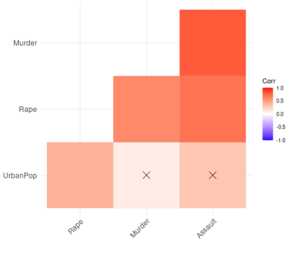
在没有显着性水平上留空

我们现在将通过在没有显着性水平的地方留空来可视化我们的相关矩阵。在前面的示例中，我们向相关矩阵添加了一个显着性水平。在这里，我们将删除相关矩阵中没有发现任何显着性水平的部分。

我们将使用 ggcorrplot函数执行此操作，并采用相关矩阵、具有 p 值的相关矩阵、hc.order、type 和 insig 等参数。

Syntax : 

ggcorrplot(correlation_matrix, hc.order=TRUE, p.mat=corrp.mat, type=”lower”, insig=”blank”)

Parameters:

correlation_matrix : Our correlation matrix to visualize.

• hc.order : If it is true, then the correlation matrix will be ordered.  
• p.mat : Correlation matrix with p-values.
• type : It is the arrangement of the character to display.
• insig : It is a character mostly containing insignificant correlation coefficients. The value is “pch” by default. If it is provided blank, then it wipes away the corresponding glyphs.

示例：在没有显着性水平上留空

电阻

library(ggplot2)
library(ggcorrplot)
  
# Reading the data
data(USArrests)
  
# Computing correlation matrix
correlation_matrix <- round(cor(USArrests),1)
  
# Computing correlation matrix with p-values
corrp.mat <- cor_pmat(USArrests)
  
# Leaving blank on no significance level
ggcorrplot(correlation_matrix, hc.order =TRUE, 
           type ="lower", p.mat = corrp.mat, insig="blank")

输出 ：