使用 Scipy – Python设计 IIR 带通 Chebyshev Type-2 滤波器

IR 代表无限脉冲响应，它是许多线性时间不变系统的显着特征之一，其特点是脉冲响应 h(t)/h(n) 在某个点后不会变为零，而是无限持续.

什么是 IIR 切比雪夫滤波器？

IIR Chebyshev 是一种与巴特沃斯一样的线性时间不变滤波器，但是，与巴特沃斯滤波器相比，它具有更陡峭的滚降。切比雪夫滤波器根据通带纹波和截止纹波等参数进一步分为切比雪夫I型和切比雪夫II型。

切比雪夫滤波器与巴特沃斯滤波器有何不同？

与巴特沃斯滤波器相比，切比雪夫滤波器具有更陡峭的滚降。

什么是切比雪夫 2 型滤波器？

Chebyshev Type-2 通过在阻带中加入相等的纹波，最大限度地减少了整个阻带上理想和实际频率响应之间的绝对差异。

规格如下：

• 通带频率：1400-2100Hz
• 阻带频率：1050-24500 Hz
• 通带纹波：0.4dB
• 阻带衰减：50 dB
• 采样频率：7 kHz

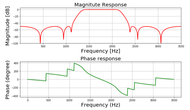
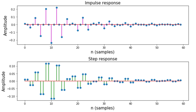
我们将绘制滤波器的幅度、相位、脉冲、阶跃响应。

循序渐进的方法：

第 1 步：导入所有必要的库。

Python3

# import required library
import numpy as np
import scipy.signal as signal
import matplotlib.pyplot as plt

步骤 2：定义用户定义函数mfreqz() 和 impz() 。 mfreqz是幅度和相位图的函数， impz是脉冲和阶跃响应的函数]

蟒蛇3

def mfreqz(b, a, Fs):
    
    # Compute frequency response of the filter
    # using signal.freqz function
    wz, hz = signal.freqz(b, a)
  
    # Calculate Magnitude from hz in dB
    Mag = 20*np.log10(abs(hz))
  
    # Calculate phase angle in degree from hz
    Phase = np.unwrap(np.arctan2(np.imag(hz), np.real(hz)))*(180/np.pi)
  
    # Calculate frequency in Hz from wz
    Freq = wz*Fs/(2*np.pi)
  
    # Plot filter magnitude and phase responses using subplot.
    fig = plt.figure(figsize=(10, 6))
  
    # Plot Magnitude response
    sub1 = plt.subplot(2, 1, 1)
    sub1.plot(Freq, Mag, 'r', linewidth=2)
    sub1.axis([1, Fs/2, -100, 5])
    sub1.set_title('Magnitute Response', fontsize=20)
    sub1.set_xlabel('Frequency [Hz]', fontsize=20)
    sub1.set_ylabel('Magnitude [dB]', fontsize=20)
    sub1.grid()
  
    # Plot phase angle
    sub2 = plt.subplot(2, 1, 2)
    sub2.plot(Freq, Phase, 'g', linewidth=2)
    sub2.set_ylabel('Phase (degree)', fontsize=20)
    sub2.set_xlabel(r'Frequency (Hz)', fontsize=20)
    sub2.set_title(r'Phase response', fontsize=20)
    sub2.grid()
  
    plt.subplots_adjust(hspace=0.5)
    fig.tight_layout()
    plt.show()
  
  
# Define impz(b,a) to calculate impulse
# response and step response of a system
# input: b= an array containing numerator
# coefficients,a= an array containing
# denominator coefficients
def impz(b, a):
  
    # Define the impulse sequence of length 60
    impulse = np.repeat(0., 60)
    impulse[0] = 1.
    x = np.arange(0, 60)
  
    # Compute the impulse response
    response = signal.lfilter(b, a, impulse)
  
    # Plot filter impulse and step response:
    fig = plt.figure(figsize=(10, 6))
    plt.subplot(211)
    plt.stem(x, response, 'm', use_line_collection=True)
    plt.ylabel('Amplitude', fontsize=15)
    plt.xlabel(r'n (samples)', fontsize=15)
    plt.title(r'Impulse response', fontsize=15)
  
    plt.subplot(212)
    step = np.cumsum(response)
  
    plt.stem(x, step, 'g', use_line_collection=True)
    plt.ylabel('Amplitude', fontsize=15)
    plt.xlabel(r'n (samples)', fontsize=15)
    plt.title(r'Step response', fontsize=15)
    plt.subplots_adjust(hspace=0.5)
  
    fig.tight_layout()
    plt.show()

第 3 步：使用给定的过滤器规格定义变量。

蟒蛇3

# Given specification
  
# Sampling frequency in Hz
Fs = 7000  
  
# Pass band frequency in Hz
fp = np.array([1400, 2100])  
  
# Stop band frequency in Hz
fs = np.array([1050, 2450])  
  
# Pass band ripple in dB
Ap = 0.4 
  
# Stop band attenuation in dB
As = 50  

步骤 4：计算截止频率

蟒蛇3

# Compute pass band and stop band edge frequencies
  
# Normalized passband edge 
# frequencies w.r.t. Nyquist rate
wp = fp/(Fs/2)  
  
# Normalized stopband 
# edge frequencies
ws = fs/(Fs/2)

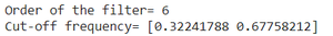
步骤 5：计算 Chebyshev 2 类数字滤波器的阶数。

蟒蛇3

# Compute order of the Chebyshev type-2
# digital filter using signal.cheb2ord
N, wc = signal.cheb2ord(wp, ws, Ap, As)
  
# Print the order of the filter
# and cutoff frequencies
print('Order of the filter=', N)
print('Cut-off frequency=', wc)

输出：

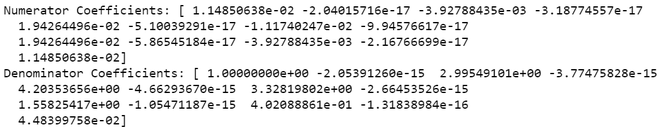
步骤 6：设计数字切比雪夫 2 型带通滤波器。

蟒蛇3

# Design digital Chebyshev type-2 bandpass 
# filter using signal.cheby2 function
z, p = signal.cheby2(N, As, wc, 'bandpass')
  
  
# Print numerator and denomerator 
# coefficients of the filter
print('Numerator Coefficients:', z)
print('Denominator Coefficients:', p)

输出：

步骤 7：绘制幅度和相位响应。

蟒蛇3

# Call mfreqz to plot the 
# magnitude and phase response
mfreqz(z, p, Fs)

输出：

步骤 8：绘制滤波器的脉冲和阶跃响应。

蟒蛇3

# Call impz function to plot impulse 
# and step response of the filter
impz(z, p)

输出：

以下是上述逐步方法的完整实现：

蟒蛇3

# import required library
import numpy as np
import scipy.signal as signal
import matplotlib.pyplot as plt
  
  
def mfreqz(b, a, Fs):
    
    # Compute frequency response of the 
    # filter using signal.freqz function
    wz, hz = signal.freqz(b, a)
  
    # Calculate Magnitude from hz in dB
  
    Mag = 20*np.log10(abs(hz))
  
    # Calculate phase angle in degree from hz
    Phase = np.unwrap(np.arctan2(np.imag(hz), np.real(hz)))*(180/np.pi)
  
    # Calculate frequency in Hz from wz
    Freq = wz*Fs/(2*np.pi)
  
    # Plot filter magnitude and phase responses using subplot.
    fig = plt.figure(figsize=(10, 6))
  
    # Plot Magnitude response
    sub1 = plt.subplot(2, 1, 1)
    sub1.plot(Freq, Mag, 'r', linewidth=2)
    sub1.axis([1, Fs/2, -100, 5])
    sub1.set_title('Magnitute Response', fontsize=20)
    sub1.set_xlabel('Frequency [Hz]', fontsize=20)
    sub1.set_ylabel('Magnitude [dB]', fontsize=20)
    sub1.grid()
  
    # Plot phase angle
    sub2 = plt.subplot(2, 1, 2)
    sub2.plot(Freq, Phase, 'g', linewidth=2)
    sub2.set_ylabel('Phase (degree)', fontsize=20)
    sub2.set_xlabel(r'Frequency (Hz)', fontsize=20)
    sub2.set_title(r'Phase response', fontsize=20)
    sub2.grid()
  
    plt.subplots_adjust(hspace=0.5)
    fig.tight_layout()
    plt.show()
  
# Define impz(b,a) to calculate impulse 
# response and step response of a system
# input: b= an array containing numerator 
# coefficients,a= an array containing 
# denominator coefficients
def impz(b, a):
    
    # Define the impulse sequence of length 60
    impulse = np.repeat(0., 60)
    impulse[0] = 1.
    x = np.arange(0, 60)
  
    # Compute the impulse response
    response = signal.lfilter(b, a, impulse)
  
    # Plot filter impulse and step response:
    fig = plt.figure(figsize=(10, 6))
    plt.subplot(211)
    plt.stem(x, response, 'm', use_line_collection=True)
    plt.ylabel('Amplitude', fontsize=15)
    plt.xlabel(r'n (samples)', fontsize=15)
    plt.title(r'Impulse response', fontsize=15)
  
    plt.subplot(212)
    step = np.cumsum(response)  
      
    # Compute step response of the system
    plt.stem(x, step, 'g', use_line_collection=True)
    plt.ylabel('Amplitude', fontsize=15)
    plt.xlabel(r'n (samples)', fontsize=15)
    plt.title(r'Step response', fontsize=15)
    plt.subplots_adjust(hspace=0.5)
  
    fig.tight_layout()
    plt.show()
  
  
# Given specification
  
# Sampling frequency in Hz
Fs = 7000  
  
# Pass band frequency in Hz
fp = np.array([1400, 2100]) 
  
# Stop band frequency in Hz
fs = np.array([1050, 2450]) 
  
# Pass band ripple in dB
Ap = 0.4 
  
# Stop band attenuation in dB
As = 50  
  
# Compute pass band and 
# stop band edge frequencies
  
# Normalized passband edge frequencies w.r.t. Nyquist rate
wp = fp/(Fs/2) 
  
# Normalized stopband edge frequencies
ws = fs/(Fs/2)  
  
# Compute order of the Chebyshev type-2 
# digital filter using signal.cheb2ord
N, wc = signal.cheb2ord(wp, ws, Ap, As)
  
# Print the order of the filter and cutoff frequencies
print('Order of the filter=', N)
print('Cut-off frequency=', wc)
  
# Design digital Chebyshev type-2 bandpass 
# filter using signal.cheby2 function
z, p = signal.cheby2(N, As, wc, 'bandpass')
  
  
# Print numerator and denomerator coefficients of the filter
print('Numerator Coefficients:', z)
print('Denominator Coefficients:', p)
  
# Call mfreqz to plot the 
# magnitude and phase response
mfreqz(z, p, Fs)
  
# Call impz function to plot impulse 
# and step response of the filter
impz(z, p)