Python中的数字带通巴特沃斯滤波器
在本文中,我们将讨论如何使用Python设计数字低通巴特沃斯滤波器。巴特沃斯滤波器是一种信号处理滤波器,旨在使通带中的频率响应尽可能平坦。让我们按照以下规格来设计滤波器并观察数字巴特沃斯滤波器的幅度、相位和脉冲响应。
什么是数字带通滤波器?
带通滤波器是一种滤波器,它通过一个范围内的频率并拒绝该范围外的频率。
它与高通和低通的区别:
通过观察带通滤波器的幅度响应可以发现主要差异。滤波器的通带具有特定范围,这意味着该范围内的唯一信号可以通过带通滤波器。任何不在指定范围内的信号都会被过滤器拒绝。
规格如下:
- 采样率为 40 kHz
- 通带边缘频率为 1400 Hz 和 2100 Hz
- 阻带边缘频率为 1050 Hz 和 2450 Hz
- 通带纹波为 0.4 dB
- 最小阻带衰减 50 dB
我们将绘制滤波器的幅度、相位和脉冲响应。
循序渐进的方法:
在开始之前,首先,我们将创建一个用户定义的函数来转换边缘频率,我们将其定义为convert()方法。
Python3
# explicit function to convert
# edge frequencies
def convertX(f_sample, f):
    w = []

    for i in range(len(f)):
        b = 2*((f[i]/2)/(f_sample/2))
        w.append(b)

    omega_mine = []

    for i in range(len(w)):
        c = (2/Td)*np.tan(w[i]/2)
        omega_mine.append(c)

    return omega_mine
Python3
# import required modules
import numpy as np
import matplotlib.pyplot as plt
from scipy import signal
import math
Python3
# Specifications of Filter

# sampling frequency
f_sample = 7000

# pass band frequency
f_pass = [1400, 2100]

# stop band frequency
f_stop = [1050, 2450]

# pass band ripple
fs = 0.5

# Sampling Time
Td = 1

# pass band ripple
g_pass = 0.4

# stop band attenuation
g_stop = 50
Python3
# Conversion to prewrapped analog
# frequency
omega_p=convertX(f_sample,f_pass)
omega_s=convertX(f_sample,f_stop)
# Design of Filter using signal.buttord
# function
N, Wn = signal.buttord(omega_p, omega_s,
g_pass, g_stop,
analog=True)
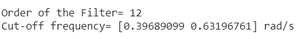
# Printing the values of order & cut-off frequency
# N is the order
print("Order of the Filter=", N)
# Wn is the cut-off freq of the filter
print("Cut-off frequency= {:} rad/s ".format(Wn))
# Conversion in Z-domain
# b is the numerator of the filter & a is
# the denominator
b, a = signal.butter(N, Wn, 'bandpass', True)
z, p = signal.bilinear(b, a, fs)
# w is the freq in z-domain & h is the
# magnitude in z-domain
w, h = signal.freqz(z, p, 512)Python3
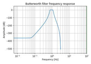
# Magnitude Response
plt.semilogx(w, 20*np.log10(abs(h)))
plt.xscale('log')
plt.title('Butterworth filter frequency response')
plt.xlabel('Frequency [Hz]')
plt.ylabel('Amplitude [dB]')
plt.margins(0, 0.1)
plt.grid(which='both', axis='both')
plt.axvline(100, color='green')
plt.show()
Python3
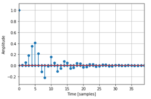
# Impulse Response
imp = signal.unit_impulse(40)
c, d = signal.butter(N, 0.5)
response = signal.lfilter(c, d, imp)

plt.stem(np.arange(0, 40), imp, markerfmt='D', use_line_collection=True)
plt.stem(np.arange(0, 40), response, use_line_collection=True)
plt.margins(0, 0.1)

plt.xlabel('Time [samples]')
plt.ylabel('Amplitude')
plt.grid(True)
plt.show()
Python3
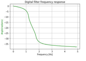
# Frequency Response
fig, ax1 = plt.subplots()
ax1.set_title('Digital filter frequency response')
ax1.set_ylabel('Angle(radians)', color='g')
ax1.set_xlabel('Frequency [Hz]')

angles = np.unwrap(np.angle(h))

ax1.plot(w/2*np.pi, angles, 'g')
ax1.grid()
ax1.axis('tight')
plt.show()
Python3
# User-defined function to convert the
# values of edge frequencies
def convertX(f_sample,f):
  w=[]

  for i in range(len(f)):
    b=2*((f[i]/2)/(f_sample/2))
    w.append(b)

  omega_mine=[]

  for i in range(len(w)):
    c=(2/Td)*np.tan(w[i]/2)
    omega_mine.append(c)

  return omega_mine

# Importing Libraries
import numpy as np
import matplotlib.pyplot as plt
from scipy import signal
import math

# Specifications of Filter

# sampling frequency
f_sample =7000

# pass band frequency
f_pass =[1400,2100]

# stop band frequency
f_stop =[1050,2450]

# pass band ripple
fs = 0.5

# Sampling Time
Td = 1

 # pass band ripple
g_pass = 0.4

# stop band attenuation
g_stop = 50

# Conversion to prewrapped analog
# frequency
omega_p=convertX(f_sample,f_pass)
omega_s=convertX(f_sample,f_stop)

# Design of Filter using signal.buttord
# function
N, Wn = signal.buttord(omega_p, omega_s,
                       g_pass, g_stop,
                       analog=True)


# Printing the values of order & cut-off frequency
# N is the order
print("Order of the Filter=", N)
# Wn is the cut-off freq of the filter
print("Cut-off frequency= {:} rad/s ".format(Wn))


# Conversion in Z-domain

# b is the numerator of the filter & a is
# the denominator
b, a = signal.butter(N, Wn, 'bandpass', True)
z, p = signal.bilinear(b, a, fs)

# w is the freq in z-domain & h is the magnitude
# in z-domain
w, h = signal.freqz(z, p, 512)

# Magnitude Response
plt.semilogx(w, 20*np.log10(abs(h)))
plt.xscale('log')
plt.title('Butterworth filter frequency response')
plt.xlabel('Frequency [Hz]')
plt.ylabel('Amplitude [dB]')
plt.margins(0, 0.1)
plt.grid(which='both', axis='both')
plt.axvline(100, color='green')
plt.show()

# Impulse Response
imp = signal.unit_impulse(40)
c, d = signal.butter(N, 0.5)
response = signal.lfilter(c, d, imp)
plt.stem(np.arange(0, 40),imp,markerfmt='D',use_line_collection=True)
plt.stem(np.arange(0,40), response,use_line_collection=True)
plt.margins(0, 0.1)
plt.xlabel('Time [samples]')
plt.ylabel('Amplitude')
plt.grid(True)
plt.show()

# Frequency Response
fig, ax1 = plt.subplots()
ax1.set_title('Digital filter frequency response')
ax1.set_ylabel('Angle(radians)', color='g')
ax1.set_xlabel('Frequency [Hz]')
angles = np.unwrap(np.angle(h))
ax1.plot(w/2*np.pi, angles, 'g')
ax1.grid()
ax1.axis('tight')
plt.show()
下面是步骤:
第 1 步:导入所有必要的库。
蟒蛇3
# import required modules
import numpy as np
import matplotlib.pyplot as plt
from scipy import signal
import math
第 2 步:使用给定的过滤器规格定义变量。
蟒蛇3
# Specifications of Filter

# sampling frequency
f_sample = 7000

# pass band frequency
f_pass = [1400, 2100]

# stop band frequency
f_stop = [1050, 2450]

# pass band ripple
fs = 0.5

# Sampling Time
Td = 1

# pass band ripple
g_pass = 0.4

# stop band attenuation
g_stop = 50
第 3 步:使用signal.buttord()函数构建过滤器。
蟒蛇3
# Conversion to prewrapped analog
# frequency
omega_p=convertX(f_sample,f_pass)
omega_s=convertX(f_sample,f_stop)

# Design of Filter using signal.buttord
# function
N, Wn = signal.buttord(omega_p, omega_s,
                       g_pass, g_stop,
                       analog=True)


# Printing the values of order & cut-off frequency
# N is the order
print("Order of the Filter=", N)

# Wn is the cut-off freq of the filter
print("Cut-off frequency= {:} rad/s ".format(Wn))


# Conversion in Z-domain

# b is the numerator of the filter & a is
# the denominator
b, a = signal.butter(N, Wn, 'bandpass', True)
z, p = signal.bilinear(b, a, fs)

# w is the freq in z-domain & h is the
# magnitude in z-domain
w, h = signal.freqz(z, p, 512)
第 4 步:绘制幅度响应。
蟒蛇3
# Magnitude Response
plt.semilogx(w, 20*np.log10(abs(h)))
plt.xscale('log')
plt.title('Butterworth filter frequency response')
plt.xlabel('Frequency [Hz]')
plt.ylabel('Amplitude [dB]')
plt.margins(0, 0.1)
plt.grid(which='both', axis='both')
plt.axvline(100, color='green')
plt.show()

第 5 步:绘制脉冲响应。
蟒蛇3
# Impulse Response
imp = signal.unit_impulse(40)
c, d = signal.butter(N, 0.5)
response = signal.lfilter(c, d, imp)

plt.stem(np.arange(0, 40), imp, markerfmt='D', use_line_collection=True)
plt.stem(np.arange(0, 40), response, use_line_collection=True)
plt.margins(0, 0.1)

plt.xlabel('Time [samples]')
plt.ylabel('Amplitude')
plt.grid(True)
plt.show()
步骤 6:绘制相位响应。
蟒蛇3
# Frequency Response
fig, ax1 = plt.subplots()
ax1.set_title('Digital filter frequency response')
ax1.set_ylabel('Angle(radians)', color='g')
ax1.set_xlabel('Frequency [Hz]')

angles = np.unwrap(np.angle(h))

ax1.plot(w/2*np.pi, angles, 'g')
ax1.grid()
ax1.axis('tight')
plt.show()

以下是基于上述方法的完整程序:
蟒蛇3
# User-defined function to convert the
# values of edge frequencies
def convertX(f_sample,f):
  w=[]

  for i in range(len(f)):
    b=2*((f[i]/2)/(f_sample/2))
    w.append(b)

  omega_mine=[]

  for i in range(len(w)):
    c=(2/Td)*np.tan(w[i]/2)
    omega_mine.append(c)

  return omega_mine

# Importing Libraries
import numpy as np
import matplotlib.pyplot as plt
from scipy import signal
import math

# Specifications of Filter

# sampling frequency
f_sample =7000

# pass band frequency
f_pass =[1400,2100]

# stop band frequency
f_stop =[1050,2450]

# pass band ripple
fs = 0.5

# Sampling Time
Td = 1

 # pass band ripple
g_pass = 0.4

# stop band attenuation
g_stop = 50

# Conversion to prewrapped analog
# frequency
omega_p=convertX(f_sample,f_pass)
omega_s=convertX(f_sample,f_stop)

# Design of Filter using signal.buttord
# function
N, Wn = signal.buttord(omega_p, omega_s,
                       g_pass, g_stop,
                       analog=True)


# Printing the values of order & cut-off frequency
# N is the order
print("Order of the Filter=", N)
# Wn is the cut-off freq of the filter
print("Cut-off frequency= {:} rad/s ".format(Wn))


# Conversion in Z-domain

# b is the numerator of the filter & a is
# the denominator
b, a = signal.butter(N, Wn, 'bandpass', True)
z, p = signal.bilinear(b, a, fs)

# w is the freq in z-domain & h is the magnitude
# in z-domain
w, h = signal.freqz(z, p, 512)

# Magnitude Response
plt.semilogx(w, 20*np.log10(abs(h)))
plt.xscale('log')
plt.title('Butterworth filter frequency response')
plt.xlabel('Frequency [Hz]')
plt.ylabel('Amplitude [dB]')
plt.margins(0, 0.1)
plt.grid(which='both', axis='both')
plt.axvline(100, color='green')
plt.show()

# Impulse Response
imp = signal.unit_impulse(40)
c, d = signal.butter(N, 0.5)
response = signal.lfilter(c, d, imp)
plt.stem(np.arange(0, 40),imp,markerfmt='D',use_line_collection=True)
plt.stem(np.arange(0,40), response,use_line_collection=True)
plt.margins(0, 0.1)
plt.xlabel('Time [samples]')
plt.ylabel('Amplitude')
plt.grid(True)
plt.show()

# Frequency Response
fig, ax1 = plt.subplots()
ax1.set_title('Digital filter frequency response')
ax1.set_ylabel('Angle(radians)', color='g')
ax1.set_xlabel('Frequency [Hz]')
angles = np.unwrap(np.angle(h))
ax1.plot(w/2*np.pi, angles, 'g')
ax1.grid()
ax1.axis('tight')
plt.show()