Python的数字低通巴特沃斯滤波器

在本文中，我们将讨论如何使用Python设计数字低通巴特沃兹滤波器。巴特沃思滤波器是一种信号处理滤波器，旨在使通带内的频率响应尽可能平坦。让我们采用以下规格来设计滤波器，并观察数字巴特沃思滤波器的幅度，相位和脉冲响应。

规格如下：

• 采样率40 kHz
• 通带边沿频率为4 kHz
• 阻带边沿频率为8kHz
• 通带纹波为0.5 dB
• 最小阻带衰减为40 dB

我们将绘制滤波器的幅度，相位和脉冲响应。

分步方法：

步骤1：导入所有必需的库。

Python3

# import required modules
import numpy as np
import matplotlib.pyplot as plt
from scipy import signal
import math

步骤2：使用过滤器的给定规格定义变量。

Python3

# Specifications of Filter
  
 # sampling frequency
f_sample = 40000 
  
# pass band frequency
f_pass = 4000  
  
# stop band frequency
f_stop = 8000  
  
# pass band ripple
fs = 0.5
  
# pass band freq in radian
wp = f_pass/(f_sample/2)  
  
# stop band freq in radian
ws = f_stop/(f_sample/2) 
  
# Sampling Time
Td = 1  
  
 # pass band ripple
g_pass = 0.5 
  
# stop band attenuation
g_stop = 40  

第三步：使用signal.buttord函数构建滤波器。

Python3

# Conversion to prewrapped analog frequency
omega_p = (2/Td)*np.tan(wp/2)
omega_s = (2/Td)*np.tan(ws/2)
  
  
# Design of Filter using signal.buttord function
N, Wn = signal.buttord(omega_p, omega_s, g_pass, g_stop, analog=True)
  
  
# Printing the values of order & cut-off frequency!
print("Order of the Filter=", N)  # N is the order
# Wn is the cut-off freq of the filter
print("Cut-off frequency= {:.3f} rad/s ".format(Wn))
  
  
# Conversion in Z-domain
  
# b is the numerator of the filter & a is the denominator
b, a = signal.butter(N, Wn, 'low', True)
z, p = signal.bilinear(b, a, fs)
# w is the freq in z-domain & h is the magnitude in z-domain
w, h = signal.freqz(z, p, 512)

输出：

步骤4：绘制幅度响应。

Python3

# Magnitude Response
plt.semilogx(w, 20*np.log10(abs(h)))
plt.xscale('log')
plt.title('Butterworth filter frequency response')
plt.xlabel('Frequency [Hz]')
plt.ylabel('Amplitude [dB]')
plt.margins(0, 0.1)
plt.grid(which='both', axis='both')
plt.axvline(100, color='green')
plt.show()

输出：

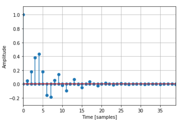
步骤5：绘制脉冲响应。

Python3

# Impulse Response
imp = signal.unit_impulse(40)
c, d = signal.butter(N, 0.5)
response = signal.lfilter(c, d, imp)
  
plt.stem(np.arange(0, 40), imp, use_line_collection=True)
plt.stem(np.arange(0, 40), response, use_line_collection=True)
plt.margins(0, 0.1)
  
plt.xlabel('Time [samples]')
plt.ylabel('Amplitude')
plt.grid(True)
plt.show()

输出：

步骤6：绘制相位响应。

Python3

# Phase Response
fig, ax1 = plt.subplots()
  
ax1.set_title('Digital filter frequency response')
ax1.set_ylabel('Angle(radians)', color='g')
ax1.set_xlabel('Frequency [Hz]')
  
angles = np.unwrap(np.angle(h))
  
ax1.plot(w/2*np.pi, angles, 'g')
ax1.grid()
ax1.axis('tight')
plt.show()

输出：

以下是基于上述方法的完整程序：

Python

# import required modules
import numpy as np
import matplotlib.pyplot as plt
from scipy import signal
import math
  
  
# Specifications of Filter
  
 # sampling frequency
f_sample = 40000 
  
# pass band frequency
f_pass = 4000  
  
# stop band frequency
f_stop = 8000  
  
# pass band ripple
fs = 0.5
  
# pass band freq in radian
wp = f_pass/(f_sample/2)  
  
# stop band freq in radian
ws = f_stop/(f_sample/2) 
  
# Sampling Time
Td = 1  
  
 # pass band ripple
g_pass = 0.5 
  
# stop band attenuation
g_stop = 40  
  
  
# Conversion to prewrapped analog frequency
omega_p = (2/Td)*np.tan(wp/2)
omega_s = (2/Td)*np.tan(ws/2)
  
  
# Design of Filter using signal.buttord function
N, Wn = signal.buttord(omega_p, omega_s, g_pass, g_stop, analog=True)
  
  
# Printing the values of order & cut-off frequency!
print("Order of the Filter=", N)  # N is the order
# Wn is the cut-off freq of the filter
print("Cut-off frequency= {:.3f} rad/s ".format(Wn))
  
  
# Conversion in Z-domain
  
# b is the numerator of the filter & a is the denominator
b, a = signal.butter(N, Wn, 'low', True)
z, p = signal.bilinear(b, a, fs)
# w is the freq in z-domain & h is the magnitude in z-domain
w, h = signal.freqz(z, p, 512)
  
  
# Magnitude Response
plt.semilogx(w, 20*np.log10(abs(h)))
plt.xscale('log')
plt.title('Butterworth filter frequency response')
plt.xlabel('Frequency [Hz]')
plt.ylabel('Amplitude [dB]')
plt.margins(0, 0.1)
plt.grid(which='both', axis='both')
plt.axvline(100, color='green')
plt.show()
  
  
# Impulse Response
imp = signal.unit_impulse(40)
c, d = signal.butter(N, 0.5)
response = signal.lfilter(c, d, imp)
plt.stem(np.arange(0, 40), imp, use_line_collection=True)
plt.stem(np.arange(0, 40), response, use_line_collection=True)
plt.margins(0, 0.1)
plt.xlabel('Time [samples]')
plt.ylabel('Amplitude')
plt.grid(True)
plt.show()
  
  
# Phase Response
fig, ax1 = plt.subplots()
ax1.set_title('Digital filter frequency response')
ax1.set_ylabel('Angle(radians)', color='g')
ax1.set_xlabel('Frequency [Hz]')
angles = np.unwrap(np.angle(h))
ax1.plot(w/2*np.pi, angles, 'g')
ax1.grid()
ax1.axis('tight')
plt.show()

输出：