使用Scipy- Python设计IIR带通椭圆滤波器

IIR代表无限冲激响应，它是许多线性时间不变系统的显着特征之一，其特征在于其冲激响应h(t)/ h(n)在任何阶段都不会达到0，而是无限期地持续存在。

什么是IIR带通椭圆滤波器?

椭圆滤波器是一种特殊类型的滤波器，当需要从通带到阻带的快速过渡时，可用于数字信号处理。

规格如下：

• 通带频率：1400-2100 Hz
• 阻带频率：1050-24500 Hz
• 通带纹波：0.4dB
• 阻带衰减：50 dB
• 采样频率：7 kHz
• 我们将绘制滤波器的幅度和相位响应。

分步方法：

步骤1：导入所有必需的库。

Python3

# import required library 
import numpy as np 
import scipy.signal as signal 
import matplotlib.pyplot as plt

步骤2：定义用户定义的函数mfreqz()和impz() 。该mfreqz为幅度和相位图的函数和impz为脉冲和阶跃响应]的函数。

Python3

# Function to depict magnitude 
# and phase plot
def mfreqz(b, a, Fs):
  
    # Compute frequency response of the
    # filter using signal.freqz function
    wz, hz = signal.freqz(b, a)
  
    # Calculate Magnitude from hz in dB
    Mag = 20*np.log10(abs(hz))
  
    # Calculate phase angle in degree from hz
    Phase = np.unwrap(np.arctan2(np.imag(hz), 
                                 np.real(hz)))*(180/np.pi)
  
    # Calculate frequency in Hz from wz
    Freq = wz*Fs/(2*np.pi)
  
    # Plot filter magnitude and phase responses using subplot.
    fig = plt.figure(figsize=(10, 6))
  
    # Plot Magnitude response
    sub1 = plt.subplot(2, 1, 1)
    sub1.plot(Freq, Mag, 'r', linewidth=2)
    sub1.axis([1, Fs/2, -100, 5])
    sub1.set_title('Magnitute Response', fontsize=20)
    sub1.set_xlabel('Frequency [Hz]', fontsize=20)
    sub1.set_ylabel('Magnitude [dB]', fontsize=20)
    sub1.grid()
  
    # Plot phase angle
    sub2 = plt.subplot(2, 1, 2)
    sub2.plot(Freq, Phase, 'g', linewidth=2)
    sub2.set_ylabel('Phase (degree)', fontsize=20)
    sub2.set_xlabel(r'Frequency (Hz)', fontsize=20)
    sub2.set_title(r'Phase response', fontsize=20)
    sub2.grid()
  
    plt.subplots_adjust(hspace=0.5)
    fig.tight_layout()
    plt.show()
  
  
# Define impz(b,a) to calculate impulse
# response and step response of a system
# input: b= an array containing numerator
# coefficients,a= an array containing
# denominator coefficients
def impz(b, a):
  
    # Define the impulse sequence of length 60
    impulse = np.repeat(0., 60)
    impulse[0] = 1.
    x = np.arange(0, 60)
  
    # Compute the impulse response
    response = signal.lfilter(b, a, impulse)
  
    # Plot filter impulse and step response:
    fig = plt.figure(figsize=(10, 6))
    plt.subplot(211)
    plt.stem(x, response, 'm', use_line_collection=True)
    plt.ylabel('Amplitude', fontsize=15)
    plt.xlabel(r'n (samples)', fontsize=15)
    plt.title(r'Impulse response', fontsize=15)
  
    plt.subplot(212)
    step = np.cumsum(response)
  
    # Compute step response of the system
    plt.stem(x, step, 'g', use_line_collection=True)
    plt.ylabel('Amplitude', fontsize=15)
    plt.xlabel(r'n (samples)', fontsize=15)
    plt.title(r'Step response', fontsize=15)
    plt.subplots_adjust(hspace=0.5)
  
    fig.tight_layout()
    plt.show()

步骤3：使用过滤器的给定规格定义变量。

Python3

# Given specification
  
# Sampling frequency in Hz
Fs = 7000
  
# Pass band frequency in Hz
fp = np.array([1400, 2100])
  
# Stop band frequency in Hz
fs = np.array([1050, 2450])
  
# Pass band ripple in dB
Ap = 0.4
  
# Stop band attenuation in dB
As = 50

步骤4：计算截止频率

Python3

# Compute pass band and stop band edge frequencies
  
# Normalized passband edge
# frequencies w.r.t. Nyquist rate
wp = fp/(Fs/2)
  
# Normalized stopband
# edge frequencies
ws = fs/(Fs/2)

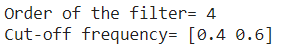
步骤5：计算椭圆带通数字滤波器的阶数。

Python3

# Compute order of the elliptic filter 
# using signal.ellipord
N, wc = signal.ellipord(wp, ws, Ap, As)
  
# Print the order of the filter and 
# cutoff frequencies
print('Order of the filter=', N)
print('Cut-off frequency=', wc)

步骤6：设计数字椭圆带通滤波器。

Python3

# Design digital elliptic bandpass filter 
# using signal.ellip function
z, p = signal.ellip(N, Ap, As, wc, 'bandpass')
  
  
# Print numerator and denomerator 
# coefficients of the filter
print('Numerator Coefficients:', z)
print('Denominator Coefficients:', p)

步骤7：绘制幅度和相位响应。

Python3

# Depicting visulalizations
  
# Call mfreqz to plot the magnitude and phase response
mfreqz(z, p, Fs)

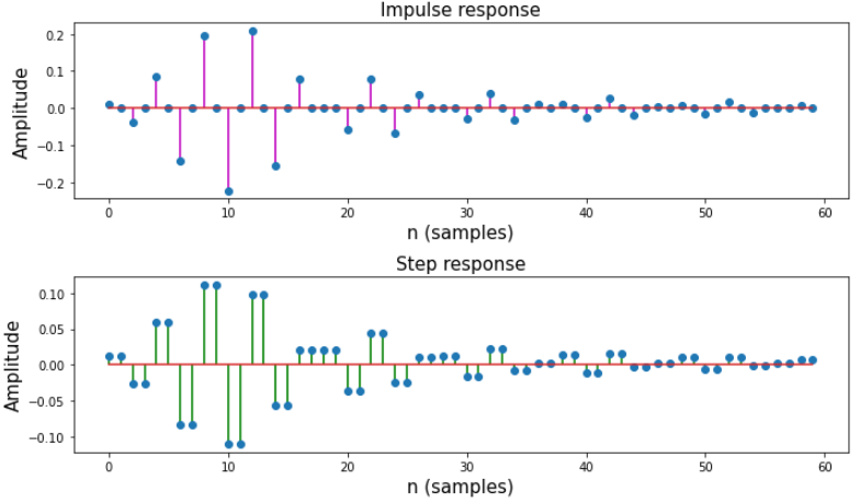
步骤8：绘制滤波器的脉冲和阶跃响应。

Python3

# Call impz function to plot impulse 
# and step response of the filter
impz(z, p)

以下是上述逐步方法的完整实现：

Python3

# Import required library
import numpy as np
import scipy.signal as signal
import matplotlib.pyplot as plt
  
  
# Function to depict magnitude 
# and phase plot
def mfreqz(b, a, Fs):
  
    # Compute frequency response of the
    # filter using signal.freqz function
    wz, hz = signal.freqz(b, a)
  
    # Calculate Magnitude from hz in dB
    Mag = 20*np.log10(abs(hz))
  
    # Calculate phase angle in degree from hz
    Phase = np.unwrap(np.arctan2(np.imag(hz), 
                                 np.real(hz)))*(180/np.pi)
  
    # Calculate frequency in Hz from wz
    Freq = wz*Fs/(2*np.pi)
  
    # Plot filter magnitude and phase responses using subplot.
    fig = plt.figure(figsize=(10, 6))
  
    # Plot Magnitude response
    sub1 = plt.subplot(2, 1, 1)
    sub1.plot(Freq, Mag, 'r', linewidth=2)
    sub1.axis([1, Fs/2, -100, 5])
    sub1.set_title('Magnitute Response', fontsize=20)
    sub1.set_xlabel('Frequency [Hz]', fontsize=20)
    sub1.set_ylabel('Magnitude [dB]', fontsize=20)
    sub1.grid()
  
    # Plot phase angle
    sub2 = plt.subplot(2, 1, 2)
    sub2.plot(Freq, Phase, 'g', linewidth=2)
    sub2.set_ylabel('Phase (degree)', fontsize=20)
    sub2.set_xlabel(r'Frequency (Hz)', fontsize=20)
    sub2.set_title(r'Phase response', fontsize=20)
    sub2.grid()
  
    plt.subplots_adjust(hspace=0.5)
    fig.tight_layout()
    plt.show()
  
  
# Define impz(b,a) to calculate impulse
# response and step response of a system
# input: b= an array containing numerator
# coefficients,a= an array containing
# denominator coefficients
def impz(b, a):
  
    # Define the impulse sequence of length 60
    impulse = np.repeat(0., 60)
    impulse[0] = 1.
    x = np.arange(0, 60)
  
    # Compute the impulse response
    response = signal.lfilter(b, a, impulse)
  
    # Plot filter impulse and step response:
    fig = plt.figure(figsize=(10, 6))
    plt.subplot(211)
    plt.stem(x, response, 'm', use_line_collection=True)
    plt.ylabel('Amplitude', fontsize=15)
    plt.xlabel(r'n (samples)', fontsize=15)
    plt.title(r'Impulse response', fontsize=15)
  
    plt.subplot(212)
    step = np.cumsum(response)
  
    # Compute step response of the system
    plt.stem(x, step, 'g', use_line_collection=True)
    plt.ylabel('Amplitude', fontsize=15)
    plt.xlabel(r'n (samples)', fontsize=15)
    plt.title(r'Step response', fontsize=15)
    plt.subplots_adjust(hspace=0.5)
  
    fig.tight_layout()
    plt.show()
  
  
# Given specification
  
# Sampling frequency in Hz
Fs = 7000
  
# Pass band frequency in Hz
fp = np.array([1400, 2100])
  
# Stop band frequency in Hz
fs = np.array([1050, 2450])
  
# Pass band ripple in dB
Ap = 0.4
  
# Stop band attenuation in dB
As = 50
  
# Compute pass band and
# stop band edge frequencies
# Normalized passband edge frequencies 
# w.r.t. Nyquist rate
wp = fp/(Fs/2)
  
# Normalized stopband edge frequencies
ws = fs/(Fs/2)
  
# Compute order of the elliptic filter 
# using signal.ellipord
N, wc = signal.ellipord(wp, ws, Ap, As)
  
# Print the order of the filter and cutoff frequencies
print('Order of the filter=', N)
print('Cut-off frequency=', wc)
  
# Design digital elliptic bandpass filter 
# using signal.ellip() function
z, p = signal.ellip(N, Ap, As, wc, 'bandpass')
  
  
# Print numerator and denomerator coefficients of the filter
print('Numerator Coefficients:', z)
print('Denominator Coefficients:', p)
  
  
# Depicting visulalizations
  
# Call mfreqz to plot the magnitude and 
# phase response
mfreqz(z, p, Fs)
# Call impz function to plot impulse and 
# step response of the filter
impz(z, p)

输出：