Python|使用 sklearn 进行线性回归
先决条件:线性回归
线性回归是一种基于监督学习的机器学习算法。它执行回归任务。回归基于自变量对目标预测值进行建模。它主要用于找出变量之间的关系和预测。不同的回归模型基于——因变量和自变量之间的关系类型、它们正在考虑的以及所使用的自变量的数量而有所不同。
本文将演示如何使用各种Python库在给定数据集上实现线性回归。我们将演示一个二元线性模型,因为这将更容易可视化。
在这个演示中,模型将使用梯度下降来学习。你可以在这里了解它。
第 1 步:导入所有必需的库
import numpy as np
import pandas as pd
import seaborn as sns
import matplotlib.pyplot as plt
from sklearn import preprocessing, svm
from sklearn.model_selection import train_test_split
from sklearn.linear_model import LinearRegression
第 2 步:读取数据集
您可以在此处下载数据集。
cd C:\Users\Dev\Desktop\Kaggle\Salinity
# Changing the file read location to the location of the dataset
df = pd.read_csv('bottle.csv')
df_binary = df[['Salnty', 'T_degC']]
# Taking only the selected two attributes from the dataset
df_binary.columns = ['Sal', 'Temp']
# Renaming the columns for easier writing of the code
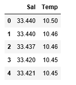
df_binary.head()
# Displaying only the 1st rows along with the column names
 第 3 步:探索数据分散
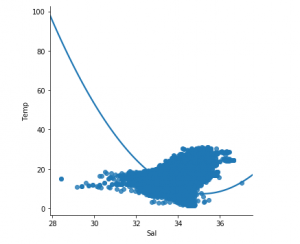
sns.lmplot(x ="Sal", y ="Temp", data = df_binary, order = 2, ci = None)

# Plotting the data scatter
 第四步:数据清洗
# Eliminating NaN or missing input numbers
df_binary.fillna(method ='ffill', inplace = True)
第 5 步:训练我们的模型
X = np.array(df_binary['Sal']).reshape(-1, 1)
y = np.array(df_binary['Temp']).reshape(-1, 1)

# Separating the data into independent and dependent variables
# Converting each dataframe into a numpy array
# since each dataframe contains only one column
df_binary.dropna(inplace = True)

# Dropping any rows with Nan values
X_train, X_test, y_train, y_test = train_test_split(X, y, test_size = 0.25)

# Splitting the data into training and testing data
regr = LinearRegression()

regr.fit(X_train, y_train)
print(regr.score(X_test, y_test))
![]() 第 6 步:探索我们的结果
第 6 步:探索我们的结果
y_pred = regr.predict(X_test)
plt.scatter(X_test, y_test, color ='b')
plt.plot(X_test, y_pred, color ='k')

plt.show()
# Data scatter of predicted values
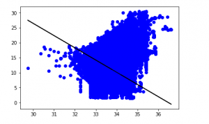
我们模型的低准确度分数表明我们的回归模型不太适合现有数据。这表明我们的数据不适合线性回归。但有时,如果我们只考虑其中的一部分,数据集可能会接受线性回归量。让我们检查一下这种可能性。第 7 步:使用较小的数据集
df_binary500 = df_binary[:][:500]

# Selecting the 1st 500 rows of the data
sns.lmplot(x ="Sal", y ="Temp", data = df_binary500,
                               order = 2, ci = None)
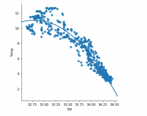
我们已经可以看到前 500 行遵循线性模型。继续执行与之前相同的步骤。
df_binary500.fillna(method ='ffill', inplace = True)

X = np.array(df_binary500['Sal']).reshape(-1, 1)
y = np.array(df_binary500['Temp']).reshape(-1, 1)

df_binary500.dropna(inplace = True)
X_train, X_test, y_train, y_test = train_test_split(X, y, test_size = 0.25)

regr = LinearRegression()
regr.fit(X_train, y_train)
print(regr.score(X_test, y_test))
![]()
y_pred = regr.predict(X_test)
plt.scatter(X_test, y_test, color ='b')
plt.plot(X_test, y_pred, color ='k')

plt.show()

在评论中写代码?请使用 ide.geeksforgeeks.org,生成链接并在此处分享链接。