决策树是使用类似于流程图的树形结构的决策工具,或者是决策及其所有可能结果(包括结果,投入成本和效用)的模型。
决策树算法属于监督学习算法的范畴。它既适用于连续变量,也适用于分类输出变量。
分支/边表示节点的结果,并且节点具有以下任一项:
- 条件[决策节点]
- 结果[终端节点]
分支/边表示语句的真实/虚假,并根据以下示例中的内容进行决策,该示例显示了一个决策树,该决策树评估三个数字中的最小数字: 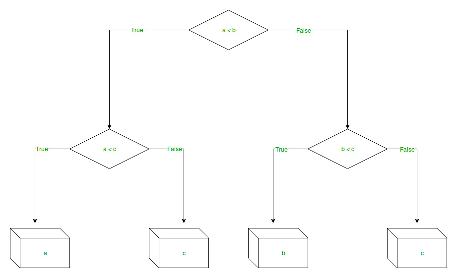
决策树回归:
决策树回归观察对象的特征,并在树的结构中训练模型,以预测将来的数据以产生有意义的连续输出。连续输出意味着输出/结果不是离散的,即,它不仅仅由离散的已知数字或值集表示。
离散输出示例:天气预报模型,用于预测特定日子是否会下雨。
连续输出示例:利润预测模型,该模型陈述了可以通过产品销售产生的可能利润。
在此,借助决策树回归模型来预测连续值。
让我们看一下分步实施–
- 步骤1:导入所需的库。
# import numpy package for arrays and stuff import numpy as np # import matplotlib.pyplot for plotting our result import matplotlib.pyplot as plt # import pandas for importing csv files import pandas as pd - 步骤2:初始化并打印数据集。
# import dataset
# dataset = pd.read_csv('Data.csv')
# alternatively open up .csv file to read data

dataset = np.array(
[['Asset Flip', 100, 1000],
['Text Based', 500, 3000],
['Visual Novel', 1500, 5000],
['2D Pixel Art', 3500, 8000],
['2D Vector Art', 5000, 6500],
['Strategy', 6000, 7000],
['First Person Shooter', 8000, 15000],
['Simulator', 9500, 20000],
['Racing', 12000, 21000],
['RPG', 14000, 25000],
['Sandbox', 15500, 27000],
['Open-World', 16500, 30000],
['MMOFPS', 25000, 52000],
['MMORPG', 30000, 80000]
])

# print the dataset
print(dataset)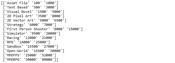
- 步骤3:从数据集中选择所有行和列1到“ X”。
# select all rows by : and column 1
# by 1:2 representing features
X = dataset[:, 1:2].astype(int)

# print X
print(X)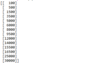
- 步骤4:从数据集中选择所有行和列2到“ y”。
# select all rows by : and column 2
# by 2 to Y representing labels
y = dataset[:, 2].astype(int)

# print y
print(y)
- 步骤5:将决策树回归器拟合到数据集
# import the regressor
from sklearn.tree import DecisionTreeRegressor

# create a regressor object
regressor = DecisionTreeRegressor(random_state = 0)

# fit the regressor with X and Y data
regressor.fit(X, y)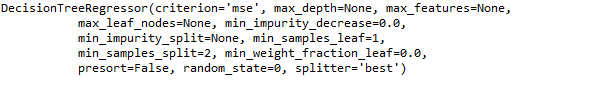
- 步骤6:预测新值
# predicting a new value

# test the output by changing values, like 3750
y_pred = regressor.predict(3750)

# print the predicted price
print("Predicted price: % d\n"% y_pred)
- 步骤7:可视化结果
# arange for creating a range of values
# from min value of X to max value of X
# with a difference of 0.01 between two
# consecutive values
X_grid = np.arange(min(X), max(X), 0.01)

# reshape for reshaping the data into
# a len(X_grid)*1 array, i.e. to make
# a column out of the X_grid values
X_grid = X_grid.reshape((len(X_grid), 1))

# scatter plot for original data
plt.scatter(X, y, color = 'red')

# plot predicted data
plt.plot(X_grid, regressor.predict(X_grid), color = 'blue')

# specify title
plt.title('Profit to Production Cost (Decision Tree Regression)')

# specify X axis label
plt.xlabel('Production Cost')

# specify Y axis label
plt.ylabel('Profit')

# show the plot
plt.show()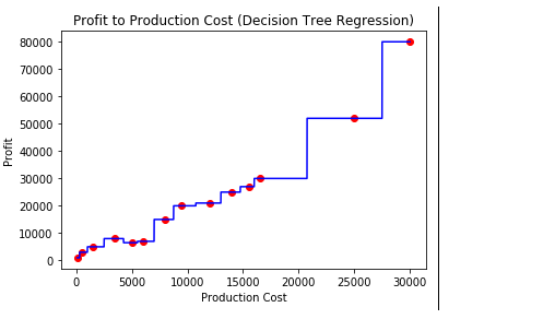
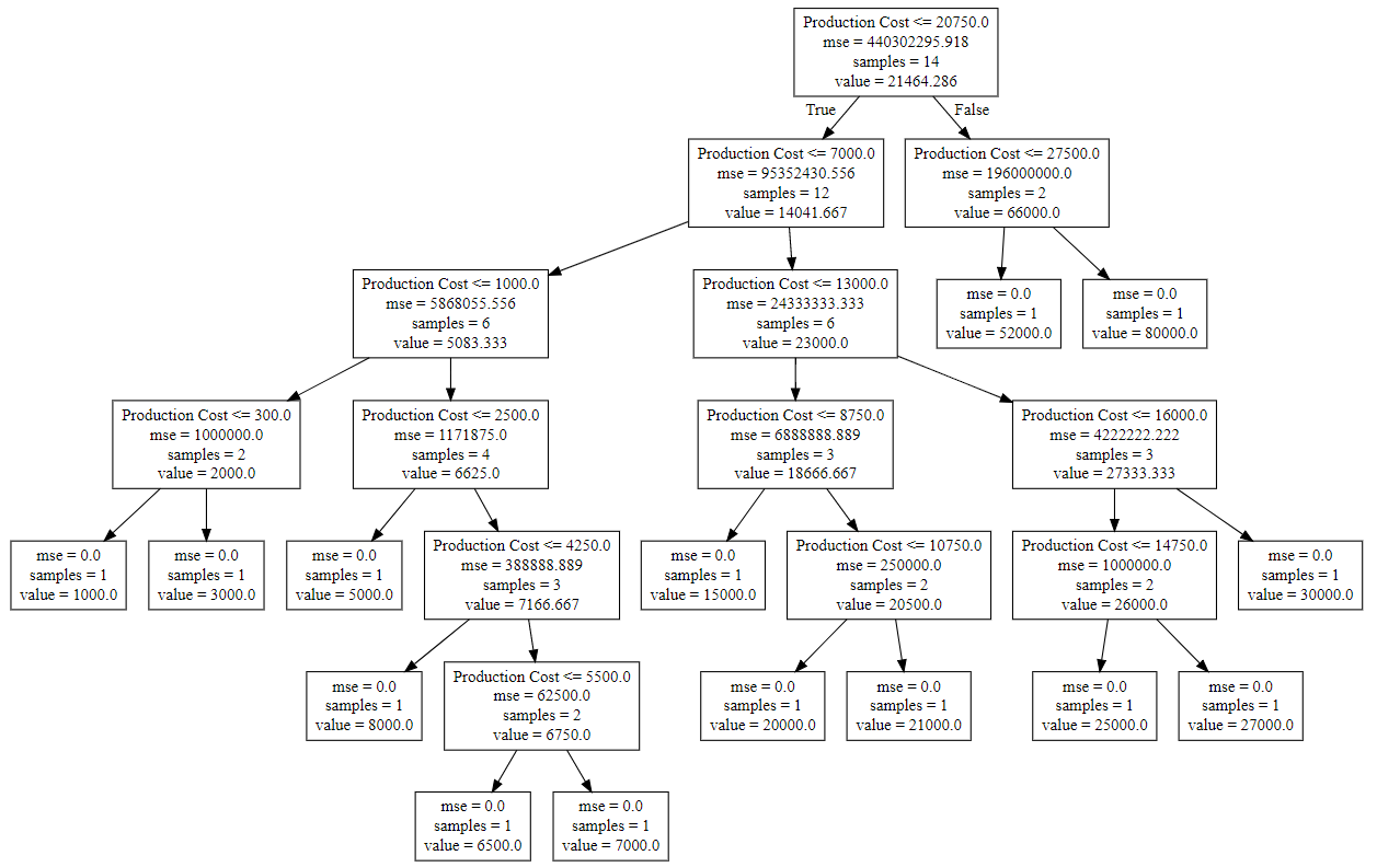
- 步骤8:最后将树导出并显示在下面的树结构中,通过复制“ tree.dot”文件中的数据,使用http://www.webgraphviz.com/对其进行可视化。
# import export_graphviz
from sklearn.tree import export_graphviz

# export the decision tree to a tree.dot file
# for visualizing the plot easily anywhere
export_graphviz(regressor, out_file ='tree.dot',
               feature_names =['Production Cost'])
输出(决策树):