R中使用ggplot2的直方图

ggplot2 是一个专用于数据可视化的 R 包。 ggplot2 包 提高图形的质量和美感（美学）。通过使用 ggplot2，我们可以在 RStudio 中制作几乎所有类型的图形

直方图是数值数据分布的近似表示。在直方图中，每个条形将数字分组到范围内。较高的条形表示更多数据落在该范围内。直方图显示连续样本数据的形状和分布。

直方图通过描述在特定值范围内发生的观察频率，粗略地让我们了解给定变量的概率分布。基本上，直方图用于显示给定变量的分布，而条形图用于比较变量。直方图绘制定量数据，数据范围按区间分组，而条形图绘制分类数据。

geom_histogram()函数是 ggplot2 模块的内置函数。

方法

• 导入模块
• 创建数据框
• 使用函数创建直方图
• 显示图

示例 1：

R

set.seed(123)
  
# In the above line,123 is set as the 
# random number value
# The main point of using the seed is to
# be able to reproduce a particular sequence 
# of 'random' numbers. and sed(n) reproduces
# random numbers results by seed
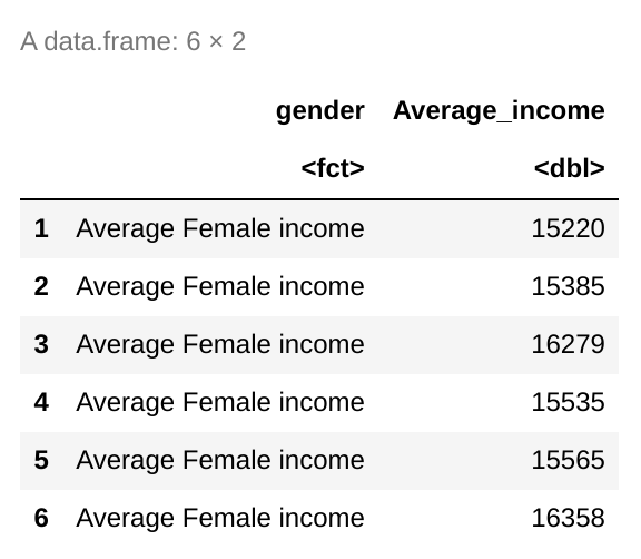
df <- data.frame(
   gender=factor(rep(c(
     "Average Female income ", "Average Male incmome"), each=20000)),
   Average_income=round(c(rnorm(20000, mean=15500, sd=500), 
                          rnorm(20000, mean=17500, sd=600)))   
)  
head(df)
  
# if already installed ggplot2 then use library(ggplot2)
library(ggplot2)
  
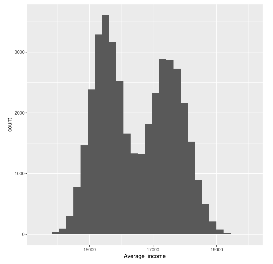
# Basic histogram
ggplot(df, aes(x=Average_income)) + geom_histogram()
  
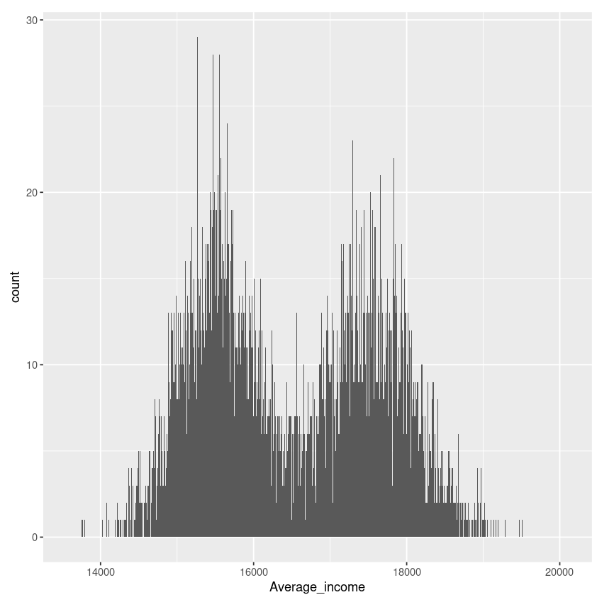
# Change the width of bins
ggplot(df, aes(x=Average_income)) +    
  
   geom_histogram(binwidth=1)
  
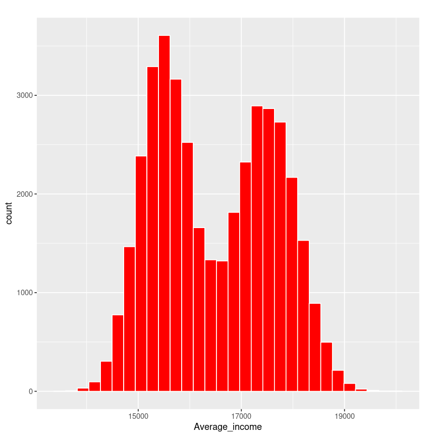
# Change colors
p<-ggplot(df, aes(x=Average_income)) +   
  
   geom_histogram(color="white", fill="red")
p

输出 ：

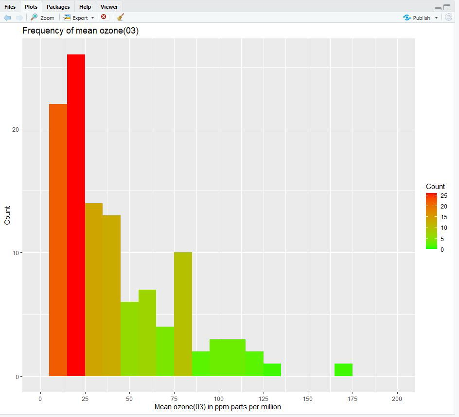
示例 2：

电阻

plot_hist <- ggplot(airquality, aes(x = Ozone)) +
  
   # binwidth help to change the thickness (Width) of the bar 
   geom_histogram(aes(fill = ..count..), binwidth = 10)+
  
   # name = "Mean ozone(03) in ppm parts per million "
   # name is used to give name to axis  
   scale_x_continuous(name = "Mean ozone(03) in ppm parts per million ",
                      breaks = seq(0, 200, 25),
                      limits=c(0, 200)) +
   scale_y_continuous(name = "Count") +
  
   # ggtitle is used to give name to a chart
   ggtitle("Frequency of mean ozone(03)") +
   scale_fill_gradient("Count", low = "green", high = "red")
  
plot_hist

输出 ：