使用六边形分箱和等高线图进行探索

六边形分箱是两个数值变量的图，其中记录分箱成六边形。下面的代码是完成平方英尺与房屋税收评估值之间关系的六边形分箱图。记录被分组到六边形箱中，而不是绘制点，颜色表示该箱中的记录数。要获取使用的 csv 文件，请单击此处。加载库

Python3

import numpy as np
import pandas as pd
import seaborn as sns
import matplotlib.pyplot as plt

加载数据中

Python3

data = pd.read_csv("kc_tax.csv")
 
print (data.head())

输出：

TaxAssessedValue  SqFtTotLiving  ZipCode
0               NaN           1730  98117.0
1          206000.0           1870  98002.0
2          303000.0           1530  98166.0
3          361000.0           2000  98108.0
4          459000.0           3150  98108.0

数据信息

Python3

print (data.shape)
print ("\n", data.info())

输出：

(498249, 3)


RangeIndex: 498249 entries, 0 to 498248
Data columns (total 3 columns):
TaxAssessedValue    497511 non-null float64
SqFtTotLiving       498249 non-null int64
ZipCode             467900 non-null float64
dtypes: float64(2), int64(1)
memory usage: 11.4 MB

选择数据

Python3

# Take a subset of the King County, Washington
# Tax data, for Assessed Value for Tax purposes
# < $600, 000 and Total Living Sq. Feet > 100 &
# < 2000
 
data = data.loc[(data['TaxAssessedValue'] < 600000) &
                (data['SqFtTotLiving'] > 100) &
                (data['SqFtTotLiving'] < 2000)]

检查空值

Python3

# As you can see in the info
# that records are not complete
data['TaxAssessedValue'].isnull().values.any()

输出：

False

代码 #1：六边形分箱

Python3

x = data['SqFtTotLiving']
y = data['TaxAssessedValue']
 
fig = sns.jointplot(x, y, kind ="hex",
                    color ="# 4CB391")
 
fig.fig.subplots_adjust(top = 0.85)
 
fig.set_axis_labels('Total Sq.Ft of Living Space',
                    'Assessed Value for Tax Purposes')
 
fig.fig.suptitle('Tax Assessed vs. Total Living Space',
                 size = 18);

输出： 等高线图：等高线图是一条曲线，两个变量的函数沿该曲线具有恒定值。它是函数f(x,y) 的三维图的平面截面，平行于 x,y 平面。等高线连接给定水平以上等高（高度）的点。等高线图是在下面的代码中说明的地图。等高线图的等高线间隔是连续等高线之间的高程差。代码 #2：等高线图

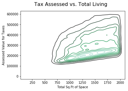
Python3

fig2 = sns.kdeplot(x, y, legend = True)
 
plt.xlabel('Total Sq.Ft of Space')
 
plt.ylabel('Assessed Value for Taxes')
 
fig2.figure.suptitle('Tax Assessed vs. Total Living', size = 16);

输出：