使用 R 编程的随机块设计

实验设计是统计学中方差分析的一部分。它们是预定义的算法，可帮助我们分析实验单元中组均值之间的差异。随机区组设计 (RBD)或随机完整区组设计是 Anova 类型的一部分。

随机区组设计：

设计实验的三个基本原则是复制、封闭和随机化。在这种类型的设计中，阻塞不是算法的一部分。实验的样本是随机的，重复被分配到每个实验单元的特定块。让我们考虑下面的一些实验，并在 R 编程中实现该实验。

实验一

在不同类型的作物中测试新肥料。作物分为 3 种不同的类型（块）。这些块再次分为 3 种肥料，用于这些作物。这个数字如下：

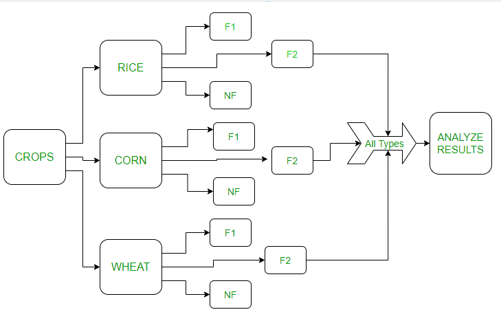
In the above image:

F1 – Fertilizer 1, F2 – Fertilizer 2 , NF – No Fertilizer  

农作物分为 3 个区块（水稻、小麦和玉米）。然后它们又被分为肥料类型。将分析不同块的结果。让我们在 R 语言中看到以上内容。

Note: In R agricolae package can also be used for implementing RCBD. But here we are using a different approach.

让我们构建数据框：

R

corn <- factor(rep(c("corn", "rice", "wheat"), each = 3))
fert <- factor(rep(c("f1", "f2", "nf"), times = 3))
corn

输出：

[1] corn  corn  corn  rice  rice  rice  wheat wheat wheat
Levels: corn rice wheat

电阻

y <- c(6, 5, 6, 
       4, 4.2, 5,
       5, 4.4, 5.5)
  
# y is the months the crops were healthy
results <- data.frame(y, corn, fert)
   
fit <- aov(y ~ fert+corn, data = results)                 
summary(fit)

输出：

Df Sum Sq Mean Sq  F value Pr(>F)  
fert         2 1.4022  0.7011   6.505 0.0553 .
corn         2 2.4156  1.2078  11.206 0.0229 *
Residuals    4 0.4311  0.1078                 
---
Signif. codes:  0 ‘***’ 0.001 ‘**’ 0.01 ‘*’ 0.05 ‘.’ 0.1 ‘ ’ 1

解释：

Mean Sq的值表明阻塞对于实验来说确实是必要的。这里 Mean Sq 0.1078<<0.7011 因此阻塞是必要的，这将为实验提供精确的值。虽然这种方法有点争议但很有用。每个实验的显着性值由进行实验的人给出。这里让我们考虑显着性有 5%，即 0.05。 Pr(>F) 值为 0.553>0.05。因此，该假设被接受用于作物实验。让我们再考虑一个实验。

实验二

比较学生（男性和女性）在不同环境（家庭和大学）中的表现。为了在图中表示此实验，如下所示：

Note: It generally is safe to consider an equal number of blocks and treatments for better results.

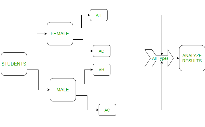
In the above image:

AC – At College, AH: At Home

学生被分为男、女两个街区。然后每个街区被分为 2 个不同的环境（家庭和大学）。让我们在代码中看到这一点：

电阻

stud <- factor(rep(c("male", "female"), each = 2))
perf <- factor(rep(c("ah", "ac" ), times = 2))
perf

输出：

[1] ah ac ah ac
Levels: ac ah

电阻

y <- c(5.5, 5,
       4, 6.2)
  
# y is the hours students 
# studied in specific places
results <- data.frame(y, stud, perf)
   
fit <- aov(y ~ perf+stud, data = results)                 
summary(fit)

输出：

Df Sum Sq Mean Sq F value Pr(>F)
perf         1 0.7225  0.7225   0.396  0.642
stud         1 0.0225  0.0225   0.012  0.930
Residuals    1 1.8225  1.8225 

解释：

Mean Sq 的值为 0.7225<<1.8225，即，这里不需要阻塞。由于 Pr 值为 0.642 > 0.05（5% 显着性），假设被接受。