了解 R 中的 t 分布

t 分布是一种概率分布，在样本量较小且总体标准差未知时对正态分布总体进行抽样时出现。它也称为学生 t 分布。它近似为钟形曲线，即近似正态分布，但峰值较低，尾部附近观测值较多。这意味着与标准正态分布或 z 分布（均值为 0，标准差为 1）相比，它为尾部提供了更高的概率。

自由度与样本大小相关，并显示可以在数据样本中自由变化的逻辑独立值的最大数量。它的计算公式为 n – 1，其中 n 是观察的总数。例如，如果您在一个样本中有 3 个观测值，其中 2 个是 10,15 并且平均值显示为 15，那么第三个观测值必须是 20。因此，在这种情况下，自由度为 2（仅两个观察结果可以自由变化）。自由度对 t 分布很重要，因为它表征曲线的形状。也就是说，t 分布的方差是根据数据集的自由度估计的。随着自由度的增加，t 分布将更接近于匹配标准正态分布，直到它们收敛（几乎相同）。因此，可以使用标准正态分布代替具有大样本量的 t 分布。

t 检验是一种统计假设检验，用于确定两组之间是否存在显着差异（差异以平均值衡量），并估计这种差异纯粹是偶然存在的可能性（p 值）。在 t 分布中，称为t-score或 t-value 的检验统计量 用于描述观测值与平均值之间的距离。 t-score 用于 t-tests 、回归测试和计算置信区间。

R 中的学生 t 分布

使用的功能：

• 要找到给定随机变量 x 的学生 t 分布的概率密度函数(pdf) 的值，请使用 R 中的dt()函数。

Syntax: dt(x, df) 

Parameters:

• x is the quantiles vector
• df is the degrees of freedom

• pt()函数用于获取 t 分布的累积分布函数(CDF)

Syntax: pt(q, df, lower.tail = TRUE)

Parameter:

• q is the quantiles vector
• df is the degrees of freedom
• lower.tail – if TRUE (default), probabilities are P[X ≤ x], otherwise, P[X > x].

• qt()函数用于获取 t 分布的分位数函数或逆累积密度函数。

Syntax: qt(p, df, lower.tail = TRUE)

Parameter:

• p is the vector of probabilities
• df is the degrees of freedom
• lower.tail – if TRUE (default), probabilities are P[X ≤ x], otherwise, P[X > x].

方法

• 设置自由度
• 要绘制学生 t 分布的密度函数，请遵循给定的步骤：
  • 首先在 R 中创建一个分位数向量。
  • 接下来，使用 dt函数找到给定随机变量 x 和特定自由度的 t 分布的值。
  • 使用这些值绘制学生 t 分布的密度函数。
• 现在，代替 dt函数，使用 pt函数获取 t 分布的累积分布函数(CDF)，使用 qt函数获取 t 分布的分位数函数或逆累积密度函数。简单地说，pt 返回 t 分布中给定随机变量 q 左侧的区域，qt 发现 t 分数是 t 分布的第 p^个分位数。

示例：要找到具有特定自由度的 x=1 处的 t 分布值，例如 D _f = 25，

R

# value of t-distribution pdf at 
# x = 0 with 25 degrees of freedom
dt(x = 1, df = 25)

输出：

0.237211

例子：

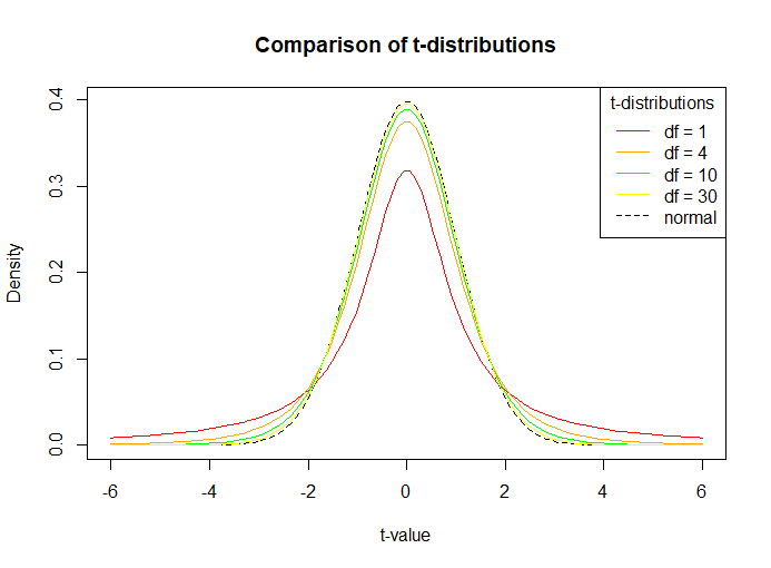
下面的代码显示了具有不同自由度的概率密度函数的比较。如前所述，样本量越大（自由度增加），图越接近正态分布（图中虚线）。

电阻

# Generate a vector of 100 values between -6 and 6
x <- seq(-6, 6, length = 100)
  
# Degrees of freedom
df = c(1,4,10,30)
colour = c("red", "orange", "green", "yellow","black")
  
# Plot a normal distribution
plot(x, dnorm(x), type = "l", lty = 2, xlab = "t-value", ylab = "Density", 
     main = "Comparison of t-distributions", col = "black")
  
# Add the t-distributions to the plot
for (i in 1:4){
  lines(x, dt(x, df[i]), col = colour[i])
}
  
# Add a legend
legend("topright", c("df = 1", "df = 4", "df = 10", "df = 30", "normal"), 
       col = colour, title = "t-distributions", lty = c(1,1,1,1,2))

输出：

示例：使用 t 分布查找 p 值和置信区间

电阻

# area to the right of a t-statistic with 
# value of 2.1 and 14 degrees of freedom
pt(q = 2.1, df = 14, lower.tail = FALSE)

输出：

0.02716657

本质上，我们发现单边 p 值 P(t>2.1) 为 2.7%。现在假设我们要构建一个双边的 95% 置信区间。为此，请使用 qt函数或分位数分布找到 95% 置信度的 t 分数或 t 值。

例子：

电阻

# value in each tail is 2.5% as confidence is 95%
# find 2.5th percentile of t-distribution with 
# 14 degrees of freedom
qt(p = 0.025, df = 14, lower.tail = TRUE)

输出：

-2.144787

因此，t 值 2.14 将用作 95% 置信区间的临界值。