毫升 |使用 PCA 实现的人脸识别

人脸识别是计算机视觉中最流行和最有争议的任务之一。使用此方法实现了最重要的里程碑之一。这种方法首先由 Sirovich 和 Kirby 于 1987 年开发，并于 1991 年由 Turk 和 Alex Pentland 首次用于人脸分类。它易于实现，因此用于许多早期的人脸识别应用程序。但它有一些注意事项，例如该算法需要具有适当光线和姿势的裁剪面部图像进行训练。在本文中，我们将讨论此方法在Python和 sklearn 中的实现。
我们需要首先导入 scikit-learn 库，以便使用该库中提供的 PCA函数API。
scikit-learn 库还提供了一个 API 来获取LFW_peoples数据集。我们还需要 matplotlib 来绘制人脸。
代码：导入库

Python3

# Import matplotlib library
import matplotlib.pyplot as plt
 
# Import scikit-learn library
from sklearn.model_selection import train_test_split
from sklearn.model_selection import GridSearchCV
from sklearn.datasets import fetch_lfw_people
from sklearn.metrics import classification_report
from sklearn.metrics import confusion_matrix
from sklearn.decomposition import PCA
from sklearn.svm import SVC
 
import numpy as np

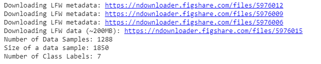
现在我们使用 sklearn 的 fetch_lfw_people函数API 导入 LFW_people 数据集。 LFW_prople 是 LFW 的预处理摘录。它包含5749类形状125 * 94的13233张图像。该函数提供了一个参数min_faces_per_person 。这个参数允许我们选择至少有 min_faces_per_person 不同图片的类。这个函数还有一个参数resize ，它可以调整提取的面部中的每个图像的大小。我们使用min_faces_per_person = 70和resize = 0.4 。
代码：

Python3

# this command will download the LFW_people's dataset to hard disk.
lfw_people = fetch_lfw_people(min_faces_per_person = 70, resize = 0.4)
 
# introspect the images arrays to find the shapes (for plotting)
n_samples, h, w = lfw_people.images.shape
 
# Instead of providing 2D data, X has data already in the form  of a vector that
# is required in this approach.
X = lfw_people.data
n_features = X.shape[1]
 
# the label to predict is the id of the person
y = lfw_people.target
target_names = lfw_people.target_names
n_classes = target_names.shape[0]
 
# Print Details about dataset
print("Number of Data Samples: % d" % n_samples)
print("Size of a data sample: % d" % n_features)
print("Number of Class Labels: % d" % n_classes)

输出：

代码：数据探索

Python3

# Function to plot images in 3 * 4 
def plot_gallery(images, titles, h, w, n_row = 3, n_col = 4):
    plt.figure(figsize =(1.8 * n_col, 2.4 * n_row))
    plt.subplots_adjust(bottom = 0, left =.01, right =.99, top =.90, hspace =.35)
    for i in range(n_row * n_col):
        plt.subplot(n_row, n_col, i + 1)
        plt.imshow(images[i].reshape((h, w)), cmap = plt.cm.gray)
        plt.title(titles[i], size = 12)
        plt.xticks(())
        plt.yticks(())
 
# Generate true labels above the images
def true_title(Y, target_names, i):
    true_name = target_names[Y[i]].rsplit(' ', 1)[-1]
    return 'true label:   % s' % (true_name)
 
true_titles = [true_title(y, target_names, i)
                     for i in range(y.shape[0])]
plot_gallery(X, true_titles, h, w)

具有真实标签的数据集样本图像

现在，我们应用 train_test_split 将数据拆分为训练集和测试集。我们使用25%的数据进行测试。
代码：拆分数据集

Python3

X_train, X_test, y_train, y_test = train_test_split(
    X, y, test_size = 0.25, random_state = 42)
print("size of training Data is % d and Testing Data is % d" %(
        y_train.shape[0], y_test.shape[0]))

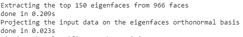
现在，我们将 PCA 算法应用于计算 EigenFaces 的训练数据集。在这里，我们取n_components = 150意味着我们从算法中提取前 150 个特征脸。我们还打印了应用此算法所花费的时间。
代码：实现 PCA

Python3

n_components = 150
 
t0 = time()
pca = PCA(n_components = n_components, svd_solver ='randomized',
          whiten = True).fit(X_train)
print("done in % 0.3fs" % (time() - t0))
 
eigenfaces = pca.components_.reshape((n_components, h, w))
 
print("Projecting the input data on the eigenfaces orthonormal basis")
t0 = time()
X_train_pca = pca.transform(X_train)
X_test_pca = pca.transform(X_test)
print("done in % 0.3fs" % (time() - t0))

上面的代码生成 EigenFace 并且每个图像由大小为1 * 150的向量表示。该向量中的值表示对应于该特征脸的系数。这些系数是使用函数上的变换函数生成的。
此 PCA 算法生成的特征脸：

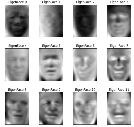
特征脸

代码：探索上述算法生成的系数。

Python3

print("Sample Data point after applying PCA\n", X_train_pca[0])
print("-----------------------------------------------------")
print("Dimensions of training set = % s and Test Set = % s"%(
        X_train.shape, X_test.shape))

Sample Data point after applying PCA 
[-2.0756025  -1.0457923   2.126936    0.03682641 -0.7575693  -0.51736575
  0.8555038   1.0519465   0.45772424  0.01348036 -0.03962574  0.63872665
  0.4816719   2.337867    1.7784412   0.13310494 -2.271292   -4.4569106
  2.0977738  -1.1379385   0.1884598  -0.33499134  1.1254574  -0.32403082
  0.14094219  1.0769527   0.7588098  -0.09976506  3.1199582   0.8837879
 -0.893391    1.1595601   1.430711    1.685587    1.3434631  -1.2590996
 -0.639135   -2.336333   -0.01364169 -1.463893   -0.46878636 -1.0548446
 -1.3329269   1.1364135   2.2223723  -1.801526   -0.3064784  -1.0281631
  4.7735424   3.4598463   1.9261417  -1.3513585  -0.2590924   2.010101
 -1.056406    0.36097565  1.1712595   0.75685936  0.90112156  0.59933555
 -0.46541685  2.0979452   1.3457304   1.9343662   5.068155   -0.70603204
  0.6064072  -0.89698195 -0.21625179 -2.1058862  -1.6839983  -0.19965973
 -1.7508434  -3.0504303   2.051207    0.39461815  0.12691127  1.2121526
 -0.79466134 -1.3895757  -2.0269105  -2.791953    1.4810398   0.1946961
  0.26118103 -0.1208623   1.1642501   0.80152154  1.2733462   0.09606536
 -0.98096275  0.31221238  1.0365396   0.8510516   0.5742255  -0.49945745
 -1.3462409  -1.036648   -0.4910289   1.0547347   1.2205439  -1.3073852
 -1.1884091   1.8626214   0.6881952   1.8356183  -1.6419449   0.57973146
  1.3768481  -1.8154184   2.0562973  -0.14337398  1.3765801  -1.4830858
 -0.0109648   2.245713    1.6913172   0.73172116  1.0212364  -0.09626482
  0.38742945 -1.8325268   0.8476424  -0.33258602 -0.96296996  0.57641584
 -1.1661777  -0.4716097   0.5479076   0.16398667  0.2818301  -0.83848953
 -1.1516216  -1.0798892  -0.58455086 -0.40767965 -0.67279476 -0.9364346
  0.62396616  0.9837545   0.1692572   0.90677387 -0.12059807  0.6222619
 -0.32074842 -1.5255395   1.3164424   0.42598936  1.2535237   0.11011053]
-----------------------------------------------------
Dimensions of training set (966, 1850) and Test Set (322, 1850)

现在我们使用支持向量机 (SVM) 作为我们的分类算法。我们使用前面步骤中生成的 PCA 系数训练数据。
代码：应用网格搜索算法

Python3

print("Fitting the classifier to the training set")
t0 = time()
param_grid = {'C': [1e3, 5e3, 1e4, 5e4, 1e5],
              'gamma': [0.0001, 0.0005, 0.001, 0.005, 0.01, 0.1], }
clf = GridSearchCV(
    SVC(kernel ='rbf', class_weight ='balanced'), param_grid
)
clf = clf.fit(X_train_pca, y_train)
print("done in % 0.3fs" % (time() - t0))
print("Best estimator found by grid search:")
print(clf.best_estimator_)
 
print("Predicting people's names on the test set")
t0 = time()
y_pred = clf.predict(X_test_pca)
print("done in % 0.3fs" % (time() - t0))
# print classification results
print(classification_report(y_test, y_pred, target_names = target_names))
# print confusion matrix
print("Confusion Matrix is:")
print(confusion_matrix(y_test, y_pred, labels = range(n_classes)))

Fitting the classifier to the training set
done in 45.872s
Best estimator found by grid search:
SVC(C=1000.0, break_ties=False, cache_size=200, class_weight='balanced',
    coef0=0.0, decision_function_shape='ovr', degree=3, gamma=0.005,
    kernel='rbf', max_iter=-1, probability=False, random_state=None,
    shrinking=True, tol=0.001, verbose=False)
Predicting people's names on the test set
done in 0.076s
                   precision    recall  f1-score   support

     Ariel Sharon       0.75      0.46      0.57        13
     Colin Powell       0.79      0.87      0.83        60
  Donald Rumsfeld       0.89      0.63      0.74        27
    George W Bush       0.84      0.98      0.90       146
Gerhard Schroeder       0.95      0.80      0.87        25
      Hugo Chavez       1.00      0.47      0.64        15
       Tony Blair       0.97      0.81      0.88        36

         accuracy                           0.85       322
        macro avg       0.88      0.72      0.77       322
     weighted avg       0.86      0.85      0.84       322

Confusion Matrix is :
[[  6   3   0   4   0   0   0]
 [  1  52   1   6   0   0   0]
 [  1   2  17   7   0   0   0]
 [  0   3   0 143   0   0   0]
 [  0   1   0   3  20   0   1]
 [  0   3   0   4   1   7   0]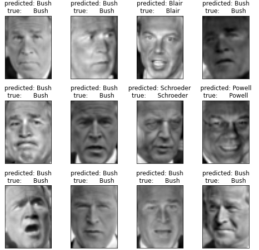
 [  0   2   1   4   0   0  29]]

所以，我们的准确度是0.85 ，我们的预测结果是：

参考：

• Scikit-learn 特征脸实现