- TensorFlow-线性回归
- TensorFlow中的线性回归(1)
- 使用Tensorflow进行线性回归
- 使用Tensorflow进行线性回归(1)
- 使用Tensorflow进行线性回归
- R线性回归(1)
- R-线性回归(1)
- R线性回归
- R-线性回归
- 线性回归 (1)
- Python线性回归(1)
- Python线性回归
- python中的线性回归(1)
- python代码示例中的线性回归
- 线性回归 - Javascript 代码示例
- 线性回归 - 无论代码示例
- 回归算法-线性回归(1)
- 回归算法-线性回归
- python 线性回归 - Python (1)
- Python中的单变量线性回归
- Python中的单变量线性回归(1)
- python 线性回归 - Python 代码示例
- 线性回归(Python实现)
- 线性回归(Python实现)(1)
- 线性回归(Python实现)
- 统计-线性回归
- 统计-线性回归(1)
- PyTorch-线性回归(1)
- PyTorch线性回归(1)
📅 最后修改于: 2021-01-11 10:38:10 🧑 作者: Mango
TensorFlow中的线性回归
线性回归是一种基于监督学习的机器学习算法。它执行回归函数。回归基于自变量对目标预测值建模。它主要用于检测变量和预测之间的关系。
线性回归是线性模型;例如,假设一个模型在输入变量(x)和单个输出变量(y)之间存在线性关系。特别地,y可以通过输入变量(x)的线性组合来计算。
线性回归是一种流行的统计方法,它使我们能够从一组连续数据中学习函数或关系。例如,我们给定x的某个数据点及其对应的数据点,我们需要知道它们之间的关系,这称为假设。
在线性回归的情况下,假设是一条直线,即
h(x)= wx + b
其中w是称为权重的向量, b是称为Bias的标量。权重和偏差称为模型参数。
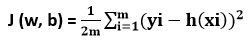
其中,m是特定数据集中的数据点。
该成本函数称为均方误差。
为了优化j值最小的参数,我们将使用一种常用的优化器算法,称为梯度下降。以下是用于梯度下降的伪代码:
Repeat until Convergence {
    w = w - ? * ?J/?w
    b = b - ? * ?J/?b
}
在哪是一个称为学习率的超参数。
线性回归的实现
我们将开始在Tensorflow中导入必要的库。我们将使用Numpy和Tensorflow进行计算,并使用Matplotlib进行绘图。
首先,我们必须导入包:
import matplotlib.pyplot as plt
import numpy as np
import tensorflow as tf
为了预测随机数,我们必须为Tensorflow和Numpy定义固定种子。
tf.set_random_seed(101)
np.random.seed(101)
现在,我们必须生成一些随机数据来训练线性回归模型。
# Generating random linear data
# There will be 50 data points which are ranging from 0 to 50.
x = np.linspace(0, 50, 50)
y = np.linspace(0, 50, 50)

# Adding noise to the random linear data
x += np.random.uniform(-4, 4, 50)
y += np.random.uniform(-4, 4, 50)
n= len(x) #Number of data points
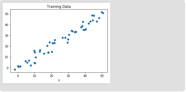
让我们可视化训练数据。
#训练数据图
plt.scatter(x, y)
plt.xlabel('x')
plt.xlabel('y')
plt.title("Training Data")
plt.show()
输出量
现在,我们将通过定义占位符x和y来开始构建模型,以便在训练过程中将训练示例x和y馈入优化器。
X= tf.placeholder("float")
Y= tf.placeholder("float")
现在,我们可以为bias和Weights声明两个可训练的TensorFlow变量,并使用方法随机初始化它们:
np.random.randn().
W= tf.Variable(np.random.randn(), name="W")
B= tf.Variable(np.random,randn(), name="b")
现在我们定义模型的超参数,学习率和时期数。
learning_rate= 0 .01
training_epochs= 1000
现在,我们将构建假设,成本函数和优化器。我们不会手动实现Gradient Decent Optimizer,因为它内置在TensorFlow中。之后,我们将在方法中初始化变量。
# Hypothesis of the function
y_pred = tf.add(tf.multiply(X, W), b)
# Mean Square Error function
      cost = tf.reduce_sum(tf.pow(y_pred-Y, 2)) / (2 * n)
# Gradient Descent Optimizer function
optimizer = tf.train.GradientDescentOptimizer (learning_rate).minimize(cost)
# Global Variables Initializer
init = tf.global_variables_initializer( )
现在我们在TensorFlow会话中开始训练过程。
# Starting the Tensorflow Session
with tf.Session() as sess:

   # Initializing the Variables
    sess.run(init)

   # Iterating through all the epochs
    for epoch in range(training_epochs):

    # Feeding each data point into the optimizer according to the Feed Dictionary.
  for (_x, _y) in zip(x, y):
  sess.run(optimizer, feed_dict = {X : _x, Y : _y})

# Here, we are displaying the result after every 50 epoch
        if (epoch + 1) % 50 ==0:
 # Calculating the cost at every epoch.
 c = sess.run(cost, feed_dict = {X : x, Y : y})
print("Epoch", (epoch + 1), ": cost =", c, "W =", sess.run(W), "b=", sess.run(b))
 # Store the necessary value which has used outside the Session
    training_cost = sess.run (cost, feed_dict ={X: x, Y: y})
    weight = sess.run(W)
    bias = sess.run(b)
输出如下:
Epoch: 50  cost = 5.8868037 W = 0.9951241 b = 1.2381057
Epoch: 100 cost = 5.7912708 W = 0.9981236 b = 1.0914398
Epoch: 150 cost = 5.7119676 W = 1.0008028 b = 0.96044315
Epoch: 200 cost = 5.6459414 W = 1.0031956 b = 0.8434396
Epoch: 250 cost = 5.590798 W = 1.0053328 b = 0.7389358
Epoch: 300 cost = 5.544609 W = 1.007242 b = 0.6455922
Epoch: 350 cost = 5.5057884 W = 1.008947 b = 0.56223
Epoch: 400 cost = 5.473068 W = 1.01047 b = 0.46775345
Epoch: 450 cost = 5.453845 W = 1.0118302 b = 0.42124168
Epoch: 500 cost = 5.421907 W = 1.0130452 b = 0.36183489
Epoch: 550 cost = 5.4019218 W = 1.0141305 b = 0.30877414
Epoch: 600 cost = 5.3848578 W = 1.0150996  b = 0.26138115
Epoch: 650 cost = 5.370247 W = 1.0159653  b = 0.21905092
Epoch: 700 cost = 5.3576995 W = 1.0167387  b = 0.18124212
Epoch: 750 cost = 5.3468934 W = 1.0174294  b = 0.14747245
Epoch: 800 cost = 5.3375574 W = 1.0180461  b = 0.11730932
Epoch: 850 cost = 5.3294765 W = 1.0185971  b = 0.090368526
Epoch: 900 cost = 5.322459 W = 1.0190894  b = 0.0663058
Epoch: 950 cost = 5.3163588 W = 1.0195289  b = 0.044813324
Epoch: 1000 cost = 5.3110332 W = 1.0199218  b = 0.02561669
现在,查看结果。
# Calculate the predictions
predictions = weight * x + bias
print ("Training cost =", training_cost, "Weight =", weight, "bias =", bias, '\n')
输出量
Training cost= 5.3110332 Weight= 1.0199214 bias=0.02561663
请注意,在这种情况下,权重和偏差都按顺序是标量。这是因为我们仅检查了训练数据中的一个因变量。如果训练数据集中有m个因变量,则权重将为一维向量,而Bias将为标量。
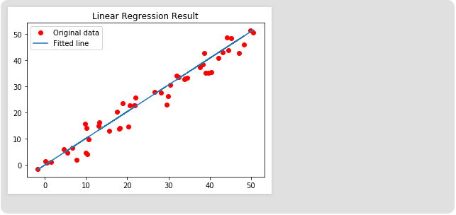
最后,我们将绘制结果:
# Plotting the Results below
plt.plot(x, y, 'ro', label ='original data')
plt.plot(x, predictions, label ='Fited line')
plt.title('Linear Regression Result')
plt.legend()
plt.show()
输出量