MATLAB多项式

📌 相关文章

📜 MATLAB多项式

📅 最后修改于: 2021-01-07 03:09:45 🧑 作者: Mango

MATLAB将多项式作为行向量执行，包括按幂次降序排列的系数。例如，方程P(X)= X ⁴ + ^7×3 – 5×+ 9可以被表示为-

p = [1 7 0 -5 9];

多项式函数

多元拟合

给定两个向量x和y，命令a = polyfit(x，y，n)通过数据点(x _i ，y _i )拟合n阶多项式，并返回(n + 1)x in的幂系数行向量系数以x的幂的降序排列，即a = [a _n a _n-1 …a ₁ a ₀ ]。

多重

给定数据向量x和行向量中多项式的系数，命令y = polyval(a，x)评估数据点x _i处的多项式并生成值y _i ，使得

y _i = a(1)x _n ⁱ + a(2)x _i ^(n-1) +…+ a(n)x + a(n + 1)。

因此，向量a的长度为n + 1，因此，求出的多项式的阶次为n。因此，如果a是5个元素长，则要求值的多项式将自动确定为四阶。

如果需要误差估计，则polyfit和polyval都使用最佳参数。

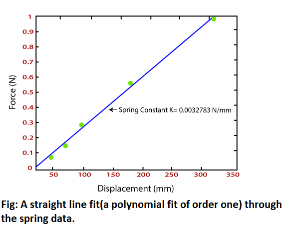
示例：直线(线性)拟合

以下数据是从旨在测量给定弹簧的弹簧常数的实验中收集的。弹簧悬挂有不同的质量m，并测量了弹簧从其未拉伸状态产生的相应偏移δ。

根据物理学，我们有F =kδ，这里F = mg。因此，我们可以从关系k = mg /δ中找到k。

在这里，我们将通过绘制实验数据，通过数据拟合最佳直线(我们知道δ和F之间的关系是线性的)，然后测量最佳拟合线的斜率来找到k。

m(g)	5.00 10.00 20.00 50.00 100.00
δ(mm)	15.5 33.07 53.39 140.24 301.03

通过数据拟合一条直线意味着我们想要找到多项式系数a ₁和₀ (一阶多项式)，使得₁ x _i + a ₀_{给出y i}的“最佳”估计。在步骤中，我们需要执行以下操作：

步骤1：找出系数a _k 's：

a = polyfit(x，y，1)

步骤2：使用拟合多项式以更精细(更紧密分布)的x _j评估y：

y_fitted = polyval(a，x_fine)

步骤3：绘制并查看。将给定输入绘制为点，将拟合数据绘制为线：

情节(x，y，'o'，x_fine，y_fitted);

以下脚本文件显示了通过弹簧实验的给定数据进行直线拟合并找到弹簧常数所包含的所有步骤。

m= [5 10 20 50 100];                % mass data (g)
d= [15 .5 33 .07 53 .39 140 .24 301 .03];        % displacement data (mm)
g=9.81;                        % g= 9.81 m/s^2
F= m/1000*g;                    % compute spring force (N)
a= polyfit (d, F, 1);                    % fit a line (1st order polynomial)
d_fit=0:10:300;                      % make a finer grid on d
F_fit=polyval (a, d_fit);                % calculate the polynomial at new points
plot (d, F,'o',d_fit,F_fit)                % plot data and the fitted curve
xlabel ('Displacement \delta (mm)'), ylabel ('Force (N)')
k=a(1);                        % Find the spring constant
text (100,.32, ['\leftarrow Spring Constant K=', num2str(k),'N/mm']);

并绘制下图：

最小二乘曲线拟合

最小二乘曲线拟合的过程可以简单地在MATLAB中实现，因为该技术产生了一组需要求解的线性方程。

大多数曲线拟合是多项式曲线拟合或指数曲线拟合(包括幂律，例如y = ax ^b )。

两个最常用的功能是：

y = ae ^bx
y = cx ^d

1.ln(y)= ln(a)+ bx或y = a ₀ + a ₁ x，其中y = ln(y)，a ₁ = b和₀ = ln?(a)。

2. ln(y)= ln(c)+ d ln(x)或y = a ₀ + a ₁ x ，其中y = ln(y)，a ₁ = d和₀ = ln?(c)。

现在我们可以在两种方法中仅使用一阶多项式来使用polyfit来确定未知常数。

涉及的步骤如下：

第1步：开发新输入：通过获取原始输入的对数，开发分配的新输入向量y和x。例如，要拟合y = ae ^bx类型的曲线，请创建

ybar = log(y)并保留x并拟合y = cx ^d类型的曲线，创建ybar = log(y)和xbar = log(x)。

步骤2：进行线性拟合：使用polyfit找出线性曲线拟合的系数a ₀和_1。

步骤3：绘制曲线：根据曲线拟合系数，计算原始常数的值(例如a，b)。根据获得的关系重新计算给定x处的y值，并绘制曲线和原始数据。

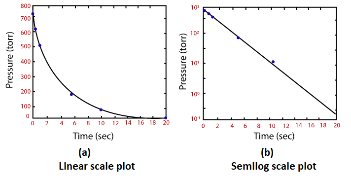
下表显示了真空泵的时间与压力变化读数。我们将通过数据拟合一条曲线P(t)= P ₀ e ^{-t /τ} ，并确定未知常数P ₀和τ。

t	0 0.5 1.0 5.0 10.0 20.0
P	760 625 528 85 14 0.16

通过记录双方关系的日志，我们可以

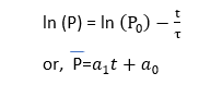
其中P = ln(P)， ₁ = MATLAB多项式 -并且₀ ＝ ln?(P ₀ )。因此，一旦我们有₁和₀ ，我们就可以很容易地计算出P ₀和τ。

示例：创建脚本文件

% EXPFIT: Exponential curve fit example
% For the following input for (t, p) fit an exponential curve
%    p=p0 * exp(-t/tau).
% The problem is resolved by taking a log and then using the linear. 
% fit (1st order polynomial)

% original input
t=[0  0.5  1  5  10  20];
p=[760  625  528  85  14  0  .16];

% Prepare new input for linear fit
tbar= t;            % no change in t is needed
pbar=log (p);            % Fit a 1st order polynomial through (tbar, pbar)
a=polyfit (tbar, pbar, 1);    % output is a=a1 a0]

% Evaluate constants p0 and tau
p0 = exp (a(2));        % a(2)=a0=log (p0)
tau=-1/a(1);            % a1=-1/tau

% (a) Plot the new curve and the input on linear scale
tnew= linspace (0, 20, 20);    % generate more refined t
pnew=p0*exp(-tnew/tau);  % calculate p at new t
plot (t, p, '0', tnew, pnew),  grid
xlabel ('Time' (sec)'), ylabel ('Pressure ((torr)')

% (b) Plot the new curve and the input on semilog scale
lpnew = exp(polyval (a, tnew));
semilogy (t, p, 'o', tnew, lpnew), grid
xlabel ('Time (sec)'), ylabel ('Pressure (torr)')

% Note: We only need one plot; we can select (a) or (b).

并绘制下图：