在 R 中用两个 Y 轴绘制图

在本文中，我们将讨论如何使用 R 编程语言创建绘图两侧的 y 轴。

有时为了快速分析数据，需要创建一个具有两个不同尺度的数据变量的图形。要在 R 语言中做到这一点，我们使用以下步骤。

首先，我们创建一个样本数据，这样样本数据由三个数值向量组成：x、y1 和 y2。 x 数据将确定 X 轴信息，而 y1 和 y2 将同时用于两个 Y 轴。

现在，我们将在散点图的左侧和右侧创建一个具有两种不同颜色和 y 轴值的散点图。为此，首先我们将在情节周围创建空白空间。这为第二个 y 轴留出空间。这可以使用 par() 方法完成。现在，围绕考虑数据 y1 的第一个 Y 轴创建第一个图（即红色十字点）。

句法：

plot(x, y1, pch , col )

接下来，在 par() 方法中将 new 设置为 TRUE。这需要在创建第一个图后再次调用。这告诉绘图将在第一个绘图上绘制新绘图。

句法：

par(new = TRUE)

接下来，考虑 y2 数据，现在绘制第二个图。

句法：

plot(x, y2, pch = 15, col = 3, axes = FALSE, xlab = “”, ylab = “”) 

如果需要，下一个设置轴或任何其他属性。

例子：

R

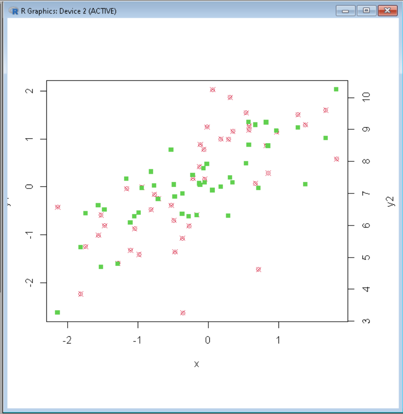
# Create sample data
set.seed(2585)                           
  
x <- rnorm(45)
y1 <- x + rnorm(45)
y2 <- x + rnorm(45, 7)
  
# Draw first plot using axis y1
par(mar = c(7, 3, 5, 4) + 0.3)              
plot(x, y1, pch = 13, col = 2)  
  
# set parameter new=True for a new axis
par(new = TRUE)         
  
# Draw second plot using axis y2
plot(x, y2, pch = 15, col = 3, axes = FALSE, xlab = "", ylab = "")
  
axis(side = 4, at = pretty(range(y2)))      
mtext("y2", side = 4, line = 3)

输出：

输出

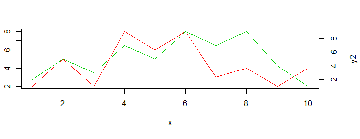
示例 2：

电阻

# Create sample data
                            
x <- c(1,2,3,4,5,6,7,8,9,10)
y1 <-c(2,5,2,8,6,8,3,4,2,4)
y2 <-c(2,5,3,7,5,9,7,9,4,1)
  
# Draw first plot using axis y1
par(mar = c(7, 3, 5, 4) + 0.3)              
plot(x, y1, type="l", col = 2)  
  
# set parameter new=True for a new axis
par(new = TRUE)         
  
# Draw second plot using axis y2
plot(x, y2, type="l", col = 3, axes = FALSE, xlab = "", ylab = "")
  
axis(side = 4, at = pretty(range(y2)))      
mtext("y2", side = 4, line = 3)

输出：