使用 Python 的 scikit-image 模块进行图像分割

将图像分成多个层的过程，由一个智能的像素级掩码表示，称为图像分割。它涉及从其集成级别合并、阻止和分离图像。将图片拆分为具有可比较属性的图像对象集合是图像处理的第一阶段。 Scikit-Image 是Python最流行的图像处理工具/模块。

安装

要安装此模块，请在终端中键入以下命令。

pip install scikit-image

转换图像格式

RGB 转灰度

skimage 包的 rgb2gray 模块用于将 3 通道 RGB 图像转换为单通道单色图像。为了应用过滤器和其他处理技术，预期输入是二维向量，即单色图像。

skimage.color.rgb2gray()函数用于将 RGB 图像转换为灰度格式

Syntax : skimage.color.rgb2gray(image)

Parameters : image : An image – RGB format

Return : The image – Grayscale format

代码：

Python3

# Importing Necessary Libraries
from skimage import data
from skimage.color import rgb2gray
import matplotlib.pyplot as plt
  
# Setting the plot size to 15,15
plt.figure(figsize=(15, 15))
  
# Sample Image of scikit-image package
coffee = data.coffee()
plt.subplot(1, 2, 1)
  
# Displaying the sample image
plt.imshow(coffee)
  
# Converting RGB image to Monochrome
gray_coffee = rgb2gray(coffee)
plt.subplot(1, 2, 2)
  
# Displaying the sample image - Monochrome
# Format
plt.imshow(gray_coffee, cmap="gray")

输出：

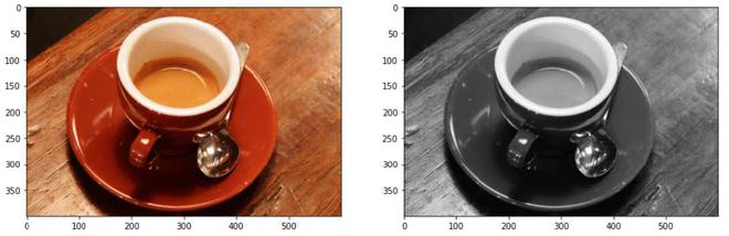
将 3 通道图像数据转换为 1 通道图像数据

说明：通过rgb2gray()函数，将形状为(400, 600, 3)的3通道RGB图像转换为形状为(400, 300)的单通道单色图像。我们将使用灰度图像来正确实现阈值函数。将每个像素的红色、绿色和蓝色像素值的平均值以获得灰度值是将彩色图片 3D 阵列转换为灰度 2D 阵列的简单方法。这通过组合每个色带的亮度或亮度贡献来创建可接受的灰度近似值。

RGB 转 HSV

HSV（色相、饱和度、值）颜色模型将 RGB 基本颜色重新映射到人类更容易理解的维度。 RGB 颜色空间描述了一种颜色中红色、绿色和蓝色的比例。在 HSV 颜色系统中，颜色是根据色调、饱和度和值来定义的。

skimage.color.rgb2hsv()函数用于将 RGB 图像转换为 HSV 格式

Syntax : skimage.color.rgb2hsv(image)

Parameters : image : An image – RGB format

Return : The image – HSV format

代码：

蟒蛇3

# Importing Necessary Libraries
from skimage import data
from skimage.color import rgb2hsv
import matplotlib.pyplot as plt
  
# Setting the plot size to 15,15
plt.figure(figsize=(15, 15))
  
# Sample Image of scikit-image package
coffee = data.coffee()
plt.subplot(1, 2, 1)
  
# Displaying the sample image
plt.imshow(coffee)
  
# Converting RGB Image to HSV Image
hsv_coffee = rgb2hsv(coffee)
plt.subplot(1, 2, 2)
  
# Displaying the sample image - HSV Format
hsv_coffee_colorbar = plt.imshow(hsv_coffee)
  
# Adjusting colorbar to fit the size of the image
plt.colorbar(hsv_coffee_colorbar, fraction=0.046, pad=0.04)

输出：

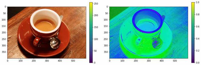
将RGB颜色格式转换为HSV颜色格式

监督分割

为了进行这种类型的分割，它需要外部输入。这包括设置阈值、转换格式和纠正外部偏差等。

通过阈值分割 - 手动输入

一个范围从 0 到 255 的外部像素值用于将图片与背景分开。这会导致修改后的图片大于或小于指定的阈值。

蟒蛇3

# Importing Necessary Libraries
# Displaying the sample image - Monochrome Format
from skimage import data
from skimage import filters
from skimage.color import rgb2gray
import matplotlib.pyplot as plt
  
# Sample Image of scikit-image package
coffee = data.coffee()
gray_coffee = rgb2gray(coffee)
  
# Setting the plot size to 15,15
plt.figure(figsize=(15, 15))
  
for i in range(10):
    
  # Iterating different thresholds
  binarized_gray = (gray_coffee > i*0.1)*1
  plt.subplot(5,2,i+1)
    
  # Rounding of the threshold
  # value to 1 decimal point
  plt.title("Threshold: >"+str(round(i*0.1,1)))
    
  # Displaying the binarized image
  # of various thresholds
  plt.imshow(binarized_gray, cmap = 'gray')
    
plt.tight_layout()

输出：

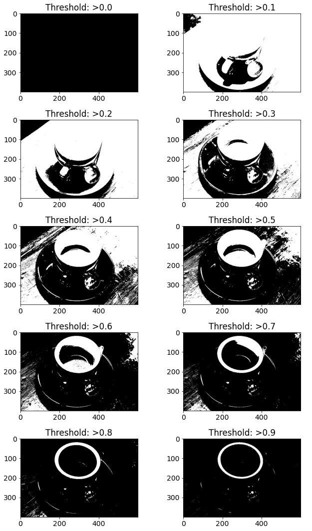
说明：此阈值的第一步是通过将图像从 0 – 255 归一化到 0 – 1 来实现的。阈值是固定的，在比较时，如果评估为真，则将结果存储为 1，否则为 0。该全局二值化图像可用于检测边缘以及分析对比度和色差。

使用 skimage.filters 模块通过阈值分割

Niblack 和 Sauvola 阈值技术专门用于提高显微图像的质量。这是一种局部阈值方法，它根据滑动窗口中每个像素的局部均值和标准差来改变阈值。 Otsu 的阈值技术通过迭代所有可能的阈值并计算阈值任一侧（即前景或背景中）样本点的离散度量来工作。目标是确定可能的最小前景和背景传播。

skimage.filters.threshold_otsu()函数用于返回基于 Otsu 方法的阈值。

Syntax : skimage.filters.threshold_otsu(image)

Parameters :

• image : An image – Monochrome format
• nbins : Number of bins required for histogram calculation
• hist : Histogram from which threshold has to be calculated

Return : threshold : Larger pixel intensity

skimage.filters.threshold_niblack()函数是一个局部阈值函数，它根据 Niblack 的方法为每个像素返回一个阈值。

Syntax : skimage.filters.threshold_niblack(image)

Parameters :

• image : An image – Monochrome format
• window_size : Window size – odd integer
• k : A positive parameter

Return : threshold : A threshold mask equal to the shape of the image

skimage.filters.threshold_sauvola()函数是一个局部阈值函数，它根据 Sauvola 的方法为每个像素返回一个阈值。

Syntax : skimage.filters.threshold_sauvola(image)

Parameters :

• image : An image – Monochrome format
• window_size : Window size – odd integer
• k : A positive parameter
• r : A postive parameter – dynamic range of standard deviation

Return : threshold : A threshold mask equal to the shape of the image

代码：

蟒蛇3

# Importing necessary libraries
from skimage import data
from skimage import filters
from skimage.color import rgb2gray
import matplotlib.pyplot as plt
  
# Setting plot size to 15, 15
plt.figure(figsize=(15, 15))
  
# Sample Image of scikit-image package
coffee = data.coffee()
gray_coffee = rgb2gray(coffee)
  
# Computing Otsu's thresholding value
threshold = filters.threshold_otsu(gray_coffee)
  
# Computing binarized values using the obtained
# thresold
binarized_coffee = (gray_coffee > threshold)*1
plt.subplot(2,2,1)
plt.title("Threshold: >"+str(threshold))
  
# Displaying the binarized image
plt.imshow(binarized_coffee, cmap = "gray")
  
# Computing Ni black's local pixel
# threshold values for every pixel
threshold = filters.threshold_niblack(gray_coffee)
  
# Computing binarized values using the obtained 
# thresold
binarized_coffee = (gray_coffee > threshold)*1
plt.subplot(2,2,2)
plt.title("Niblack Thresholding")
  
# Displaying the binarized image
plt.imshow(binarized_coffee, cmap = "gray")
  
# Computing Sauvola's local pixel threshold
# values for every pixel - Not Binarized
threshold = filters.threshold_sauvola(gray_coffee)
plt.subplot(2,2,3)
plt.title("Sauvola Thresholding")
  
# Displaying the local threshold values
plt.imshow(threshold, cmap = "gray")
  
# Computing Sauvola's local pixel
# threshold values for every pixel - Binarized
binarized_coffee = (gray_coffee > threshold)*1
plt.subplot(2,2,4)
plt.title("Sauvola Thresholding - Converting to 0's and 1's")
  
# Displaying the binarized image
plt.imshow(binarized_coffee, cmap = "gray")

输出：

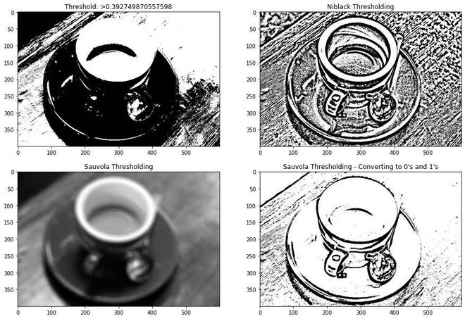
说明：这些局部阈值技术使用均值和标准差作为其主要计算参数。它们的最终局部像素值也受到其他正参数的影响。这样做是为了确保对象和背景之间的分离。

$Sauvola_{value} = \bar x * (1 + k * (\frac{\sigma}{r-1}))$

$Niblack_{value} = \bar x + k * \sigma - c$

其中 \bar x 和 \sigma 分别代表像素强度的均值和标准差。

主动轮廓分割

能量函数归约的概念是活动轮廓法的基础。活动轮廓是一种分割方法，它使用能量和限制将感兴趣的像素与图片的其余部分分开，以便进一步处理和分析。术语“活动轮廓”是指分割过程中的模型。

skimage.segmentation.active_contour（）通过拟合蛇图像特征函数主动轮廓。

Syntax : skimage.segmentation.active_contour(image, snake)

Parameters :

• image : An image
• snake : Initial snake coordinates – for bounding the feature
• alpha : Snake length shape
• beta : Snake smoothness shape
• w_line : Controls attraction – Brightness
• w_edge : Controls attraction – Edges
• gamma : Explicit time step

Return : snake : Optimised snake with input parameter’s size

代码：

蟒蛇3

# Importing necessary libraries
import numpy as np
import matplotlib.pyplot as plt
from skimage.color import rgb2gray
from skimage import data
from skimage.filters import gaussian
from skimage.segmentation import active_contour
  
# Sample Image of scikit-image package
astronaut = data.astronaut()
gray_astronaut = rgb2gray(astronaut)
  
# Applying Gaussian Filter to remove noise
gray_astronaut_noiseless = gaussian(gray_astronaut, 1)
  
# Localising the circle's center at 220, 110
x1 = 220 + 100*np.cos(np.linspace(0, 2*np.pi, 500))
x2 = 100 + 100*np.sin(np.linspace(0, 2*np.pi, 500))
  
# Generating a circle based on x1, x2
snake = np.array([x1, x2]).T
  
# Computing the Active Contour for the given image
astronaut_snake = active_contour(gray_astronaut_noiseless,
                                 snake)
  
fig = plt.figure(figsize=(10, 10))
  
# Adding subplots to display the markers
ax = fig.add_subplot(111)
  
# Plotting sample image
ax.imshow(gray_astronaut_noiseless)
  
# Plotting the face boundary marker
ax.plot(astronaut_snake[:, 0],
        astronaut_snake[:, 1], 
        '-b', lw=5)
  
# Plotting the circle around face
ax.plot(snake[:, 0], snake[:, 1], '--r', lw=5)

输出：

说明：活动轮廓模型是图像分割中的动态方法之一，它使用图像的能量限制和压力来分离感兴趣的区域。对于分割，活动轮廓为目标对象的每个部分建立不同的边界或曲率。活动轮廓模型是一种使由外力和内力产生的能量函数最小化的技术。外力被指定为曲线或曲面，而内力被定义为图片数据。外力是一种使初始轮廓自动转化为图片中物体形式的力。

Chan-Vese 分割

著名的 Chan-Vese 迭代分割方法将图片分成具有最低类内方差的两组。该算法使用迭代进化以最小化能量的集合，其特征在于对应于分割区域外整体平均值的强度变化总和的权重，特征向量内与整体平均值的差异总和，以及一项这与碎片区域边缘的长度成正比。

skimage.segmentation.chan_vese()函数用于使用边界未明确定义的 Chan-Vese 算法分割对象。

Syntax : skimage.segmentation.chan_vese(image)

Parameters :

• image : An image
• mu : Weight – Edge Length
• lambda1 : Weight – Difference from average
• tol : Tolerance of Level set variation
• max_num_iter : Maximum number of iterations
• extended_output : Tuple of 3 values is returned

Return :

• segmentation : Segmented Image
• phi : Final level set
• energies: Shows the evolution of the energy

代码：

蟒蛇3

import matplotlib.pyplot as plt
from skimage.color import rgb2gray
from skimage import data, img_as_float
from skimage.segmentation import chan_vese
fig, axes = plt.subplots(1, 3, figsize=(10, 10))
  
# Sample Image of scikit-image package
astronaut = data.astronaut()
gray_astronaut = rgb2gray(astronaut)
  
# Computing the Chan VESE segmentation technique
chanvese_gray_astronaut = chan_vese(gray_astronaut,
                                    max_iter=100,
                                    extended_output=True)
  
ax = axes.flatten()
  
# Plotting the original image
ax[0].imshow(gray_astronaut, cmap="gray")
ax[0].set_title("Original Image")
  
# Plotting the segemented - 100 iterations image
ax[1].imshow(chanvese_gray_astronaut[0], cmap="gray")
title = "Chan-Vese segmentation - {} iterations".
format(len(chanvese_gray_astronaut[2]))
  
ax[1].set_title(title)
  
# Plotting the final level set
ax[2].imshow(chanvese_gray_astronaut[1], cmap="gray")
ax[2].set_title("Final Level Set")
plt.show()

输出：

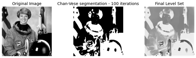
说明：活动轮廓的 Chan-Vese 模型是一种强大且通用的方法，可用于分割各种图片，包括使用“传统”方法（例如阈值法或基于梯度的方法）难以分割的一些图片。该模型常用于医学成像，特别是用于大脑、心脏和气管分割。该模型基于能量最小化问题，该问题可以在水平集公式中重铸，以使问题更容易解决。

无监督分割

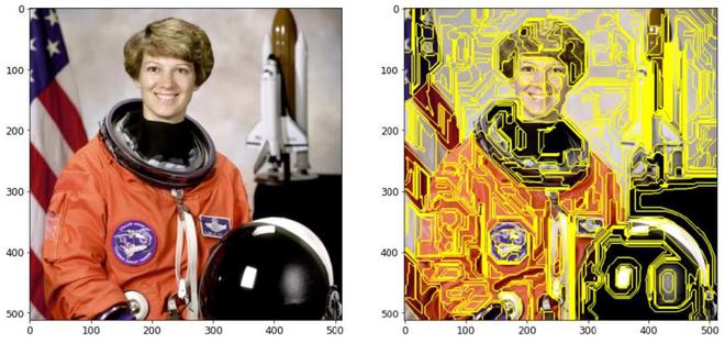
标记边界

该技术生成的图像在标记区域之间具有突出显示的边界，其中使用 SLIC 方法对图片进行分割。

skimage.segmentation.mark_boundaries()函数用于返回带有标记区域之间边界的图像。

Syntax : skimage.segmentation.mark_boundaries(image)

Parameters :

• image : An image
• label_img : Label array with marked regions
• color : RGB color of boundaries
• outline_color : RGB color of surrounding boundaries

Return : marked : An image with boundaries are marked

代码：

蟒蛇3

# Importing required boundaries
from skimage.segmentation import slic, mark_boundaries
from skimage.data import astronaut
  
# Setting the plot figure as 15, 15
plt.figure(figsize=(15, 15))
  
# Sample Image of scikit-image package
astronaut = astronaut()
  
# Applying SLIC segmentation
# for the edges to be drawn over
astronaut_segments = slic(astronaut,
                          n_segments=100,
                          compactness=1)
  
plt.subplot(1, 2, 1)
  
# Plotting the original image
plt.imshow(astronaut)
  
# Detecting boundaries for labels
plt.subplot(1, 2, 2)
  
# Plotting the ouput of marked_boundaries
# function i.e. the image with segmented boundaries
plt.imshow(mark_boundaries(astronaut, astronaut_segments))

输出：

说明：我们将图像聚类为 100 个紧凑度 = 1 的片段，这个分割的图像将作为 mark_boundaries()函数的标记数组。聚类图像的每一段由一个整数值区分，mark_boundaries 的结果是标签之间的叠加边界。

简单线性迭代聚类

通过基于颜色相似性和接近度组合图像平面中的像素，该方法生成超像素。 Simple Linear Iterative Clustering 是最先进的超像素分割方法，而且它只需要很少的计算能力。简而言之，该技术将像素聚集在五维颜色和图像平面空间中，以创建小的、几乎均匀的超像素。

skimage.segmentation.slic()函数用于使用 k-means 聚类对图像进行分割。

Syntax : skimage.segmentation.slic(image)

Parameters :

• image : An image
• n_segments : Number of labels
• compactness : Balances color and space proximity.
• max_num_iter : Maximum number of iterations

Return : labels: Integer mask indicating segment labels.

代码：

蟒蛇3

# Importing required libraries
from skimage.segmentation import slic
from skimage.data import astronaut
from skimage.color import label2rgb
  
# Setting the plot size as 15, 15
plt.figure(figsize=(15,15))
  
# Sample Image of scikit-image package
astronaut = astronaut()
  
# Applying Simple Linear Iterative
# Clustering on the image
# - 50 segments & compactness = 10
astronaut_segments = slic(astronaut,
                          n_segments=50,
                          compactness=10)
plt.subplot(1,2,1)
  
# Plotting the original image
plt.imshow(astronaut)
plt.subplot(1,2,2)
  
# Converts a label image into
# an RGB color image for visualizing
# the labeled regions. 
plt.imshow(label2rgb(astronaut_segments,
                     astronaut,
                     kind = 'avg'))

输出：

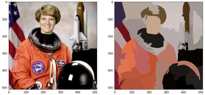
说明：此技术通过根据颜色相似性和接近程度对图片平面中的像素进行分组来创建超像素。这是在 5-D 空间中完成的，其中 XY 是像素位置。因为CIELAB空间中两种颜色之间的最大可能距离受到限制，而XY平面上的空间距离取决于图片尺寸，我们必须对空间距离进行归一化，以便在这个5D空间中应用欧几里得距离。因此，创建了一个考虑超像素大小的新距离度量，以在这个 5D 空间中聚类像素。

Felzenszwalb 的分割

计算 Felsenszwalb 的高效基于图形的图片分割。它使用快速、最小的基于生成树的聚类在图像网格上生成 RGB 图片的过度分割。这可用于隔离特征和识别边缘。该算法使用像素之间的欧几里德距离。 skimage.segmentation.felzenszwalb()函数用于计算 Felsenszwalb 的高效基于图形的图像分割。

Syntax : skimage.segmentation.felzenszwalb(image)

Parameters :

• image : An input image
• scale : Higher value – larger clusters
• sigma : Width of Gaussian kernel
• min_size : Minimum component size

Return : segment_mask : Integer mask indicating segment labels.

代码：

蟒蛇3

# Importing the required libraries
from skimage.segmentation import felzenszwalb
from skimage.color import label2rgb
from skimage.data import astronaut
  
# Setting the figure size as 15, 15
plt.figure(figsize=(15,15))
  
# Sample Image of scikit-image package
astronaut = astronaut()
  
# computing the Felzenszwalb's
# Segmentation with sigma = 5 and minimum
# size = 100
astronaut_segments = felzenszwalb(astronaut,
                                  scale = 2,
                                  sigma=5,
                                  min_size=100)
  
# Plotting the original image
plt.subplot(1,2,1)
plt.imshow(astronaut)
  
# Marking the boundaries of
# Felzenszwalb's segmentations
plt.subplot(1,2,2)
plt.imshow(mark_boundaries(astronaut,
                           astronaut_segments))

输出：

使用 mark_boundaries()函数

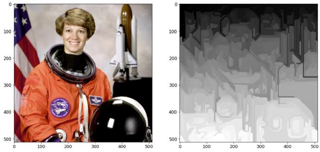
没有 mark_boundaries()函数

说明：在图片网格上使用快速、最小的基于树结构的聚类，创建多通道图像的过度分割。参数尺度决定了观察的水平。越来越少的零件与更大的规模相关联。一个高斯核的直径为 sigma，用于在分割前对图片进行平滑处理。比例是控制生成段的数量及其大小的唯一方法。图片中各个片段的大小可能会根据局部对比度发生显着变化。

还有许多其他有监督和无监督的图像分割技术。这在限制单个特征、前景隔离、降噪方面非常有用，并且有助于更直观地分析图像。在构建神经网络模型之前对图像进行分割以产生有效的结果是一种很好的做法。