📌 相关文章
- Elasticsearch-汇总数据
- Elasticsearch-汇总数据(1)
- MySQL汇总
- MySQL汇总(1)
- 如何在 R 中使用汇总函数?
- 如何汇总数据但保留列 - R 编程语言(1)
- 大数据与数据分析之间的区别
- 大数据和数据分析之间的区别(1)
- 大数据和数据分析之间的区别
- 大数据与数据分析之间的区别(1)
- 大数据和数据分析之间的区别
- 大数据和数据分析之间的区别(1)
- 数据分析和数据分析的区别(1)
- 数据分析和数据分析的区别
- Excel数据透视表-汇总值(1)
- Excel数据透视表-汇总值
- 如何汇总数据但保留列 - R 编程语言代码示例
- MS Access-汇总数据
- MS Access-汇总数据(1)
- 大数据分析-数据分析工具(1)
- 大数据分析-数据分析工具
- pandas 汇总所有列 - Python (1)
- 大数据分析-数据可视化(1)
- 大数据分析-数据可视化
- 数据分析的使用(1)
- 数据分析的使用
- 大数据分析-数据收集(1)
- 大数据分析-数据收集
- 大数据分析-数据分析师
📜 大数据分析-汇总数据
📅 最后修改于: 2020-12-02 06:39:55 🧑 作者: Mango
报告在大数据分析中非常重要。每个组织必须定期提供信息以支持其决策过程。这项任务通常由具有SQL和ETL(提取,传输和加载)经验的数据分析师处理。
负责此任务的团队负责将大数据分析部门产生的信息传播到组织的不同区域。
下面的示例演示数据汇总的含义。导航到bda / part1 / summarize_data文件夹,然后在该文件夹内部,双击打开summary_data.Rproj文件。然后,打开summary_data.R脚本并看一下代码,然后按照给出的说明进行操作。
# Install the following packages by running the following code in R.
pkgs = c('data.table', 'ggplot2', 'nycflights13', 'reshape2')
install.packages(pkgs)
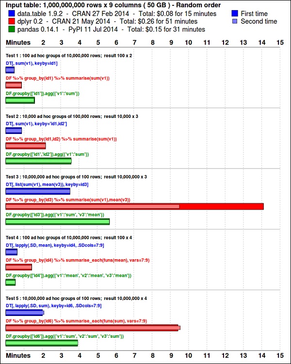
ggplot2软件包非常适合数据可视化。 data.table包是在R中进行快速且内存有效的汇总的绝佳选择。最新的基准测试表明,它甚至比用于类似任务的Python库pandas还要快。
使用以下代码查看数据。该代码也可在bda / part1 / summarize_data / summarize_data.Rproj文件中找到。
library(nycflights13)
library(ggplot2)
library(data.table)
library(reshape2)

# Convert the flights data.frame to a data.table object and call it DT
DT
以下代码有一个数据汇总的示例。
### Data Summarization
# Compute the mean arrival delay
DT[, list(mean_arrival_delay = mean(arr_delay, na.rm = TRUE))]
#        mean_arrival_delay
# 1:           6.895377
# Now, we compute the same value but for each carrier
mean1 = DT[, list(mean_arrival_delay = mean(arr_delay, na.rm = TRUE)),
   by = carrier]
print(mean1)
#      carrier    mean_arrival_delay
# 1:      UA          3.5580111
# 2:      AA          0.3642909
# 3:      B6          9.4579733
# 4:      DL          1.6443409
# 5:      EV         15.7964311
# 6:      MQ         10.7747334
# 7:      US          2.1295951
# 8:      WN          9.6491199
# 9:      VX          1.7644644
# 10:     FL         20.1159055
# 11:     AS         -9.9308886
# 12:     9E          7.3796692
# 13:     F9         21.9207048
# 14:     HA         -6.9152047
# 15:     YV         15.5569853
# 16:     OO         11.9310345

# Now let’s compute to means in the same line of code
mean2 = DT[, list(mean_departure_delay = mean(dep_delay, na.rm = TRUE),
   mean_arrival_delay = mean(arr_delay, na.rm = TRUE)),
   by = carrier]
print(mean2)

#       carrier    mean_departure_delay   mean_arrival_delay
# 1:      UA            12.106073          3.5580111
# 2:      AA             8.586016          0.3642909
# 3:      B6            13.022522          9.4579733
# 4:      DL             9.264505          1.6443409
# 5:      EV            19.955390         15.7964311
# 6:      MQ            10.552041         10.7747334
# 7:      US             3.782418          2.1295951
# 8:      WN            17.711744          9.6491199
# 9:      VX            12.869421          1.7644644
# 10:     FL            18.726075         20.1159055
# 11:     AS             5.804775         -9.9308886
# 12:     9E            16.725769          7.3796692
# 13:     F9            20.215543         21.9207048
# 14:     HA             4.900585         -6.9152047
# 15:     YV            18.996330         15.5569853
# 16:     OO            12.586207         11.9310345

### Create a new variable called gain
# this is the difference between arrival delay and departure delay
DT[, gain:= arr_delay - dep_delay]

# Compute the median gain per carrier
median_gain = DT[, median(gain, na.rm = TRUE), by = carrier]
print(median_gain)