使用Python从零开始实现线性回归

线性回归是一种监督学习算法，它既是统计算法又是机器学习算法。它用于根据给定的输入值 x 预测实值输出 y。它描述了因变量 y 和自变量 x _i （或特征）之间的关系。用于预测的假设函数由 h( x ) 表示。

h( x ) = w * x + b  
    
  here, b is the bias.
  x represents the feature vector
  w represents the weight vector.

具有一个变量的线性回归也称为单变量线性回归。初始化权重向量后，我们可以通过普通最小二乘法或梯度下降学习找到最适合模型的权重向量。

数学直觉：成本函数（或损失函数）用于衡量机器学习模型的性能或量化预期值与我们假设函数预测值之间的误差。线性回归的成本函数由 J 表示。

$\frac{1}{m} \sum_{i=1}^{m}\left(y^{(i)}-h\left(x^{(i)}\right)\right)^{2}$

Here, m is the total number of training examples in the dataset.
y(i) represents the value of target variable for ith training example.

因此，我们的目标是最小化成本函数J （或提高我们机器学习模型的性能）。为此，我们必须找到J最小的权重。一种可用于最小化任何可微函数的算法是梯度下降。它是一种一阶迭代优化算法，可将我们带到函数的最小值。

梯度下降：

伪代码：

1. 从一些 w 开始
2. 不断改变 w 以减少 J( w ) 直到我们希望最终达到最小值。

算法：

repeat until convergence  {
       tmpi = wi - alpha * dwi          
       wi = tmpi              
}
where alpha is the learning rate.

执行：

此实现中使用的数据集可以从链接下载。

它有 2 列——“ YearsExperience ”和“ Salary ”，适用于一家公司的 30 名员工。所以在这里，我们将训练一个线性回归模型来学习每个员工的工作年限与其各自工资之间的相关性。一旦模型经过训练，我们将能够根据员工多年的经验预测其薪水。

Python3

# Importing libraries
  
import numpy as np
  
import pandas as pd
  
from sklearn.model_selection import train_test_split
  
import matplotlib.pyplot as plt
  
# Linear Regression
  
class LinearRegression() :
      
    def __init__( self, learning_rate, iterations ) :
          
        self.learning_rate = learning_rate
          
        self.iterations = iterations
          
    # Function for model training
              
    def fit( self, X, Y ) :
          
        # no_of_training_examples, no_of_features
          
        self.m, self.n = X.shape
          
        # weight initialization
          
        self.W = np.zeros( self.n )
          
        self.b = 0
          
        self.X = X
          
        self.Y = Y
          
          
        # gradient descent learning
                  
        for i in range( self.iterations ) :
              
            self.update_weights()
              
        return self
      
    # Helper function to update weights in gradient descent
      
    def update_weights( self ) :
             
        Y_pred = self.predict( self.X )
          
        # calculate gradients  
      
        dW = - ( 2 * ( self.X.T ).dot( self.Y - Y_pred )  ) / self.m
       
        db = - 2 * np.sum( self.Y - Y_pred ) / self.m 
          
        # update weights
      
        self.W = self.W - self.learning_rate * dW
      
        self.b = self.b - self.learning_rate * db
          
        return self
      
    # Hypothetical function  h( x ) 
      
    def predict( self, X ) :
      
        return X.dot( self.W ) + self.b
     
  
# driver code
  
def main() :
      
    # Importing dataset
      
    df = pd.read_csv( "salary_data.csv" )
  
    X = df.iloc[:,:-1].values
  
    Y = df.iloc[:,1].values
      
    # Splitting dataset into train and test set
  
    X_train, X_test, Y_train, Y_test = train_test_split( 
      X, Y, test_size = 1/3, random_state = 0 )
      
    # Model training
      
    model = LinearRegression( iterations = 1000, learning_rate = 0.01 )
  
    model.fit( X_train, Y_train )
      
    # Prediction on test set
  
    Y_pred = model.predict( X_test )
      
    print( "Predicted values ", np.round( Y_pred[:3], 2 ) ) 
      
    print( "Real values      ", Y_test[:3] )
      
    print( "Trained W        ", round( model.W[0], 2 ) )
      
    print( "Trained b        ", round( model.b, 2 ) )
      
    # Visualization on test set 
      
    plt.scatter( X_test, Y_test, color = 'blue' )
      
    plt.plot( X_test, Y_pred, color = 'orange' )
      
    plt.title( 'Salary vs Experience' )
      
    plt.xlabel( 'Years of Experience' )
      
    plt.ylabel( 'Salary' )
      
    plt.show()
     
if __name__ == "__main__" : 
      
    main()

输出：

Predicted values  [ 40594.69 123305.18  65031.88]
Real values       [ 37731 122391  57081]
Trained W         9398.92
Trained b         26496.31

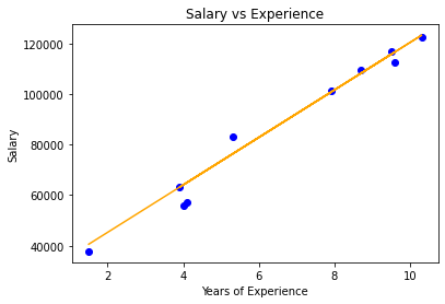
线性回归可视化