Networkx 中的有向图、多重图和可视化
先决条件:图形的基本可视化技术
在上一篇文章中,我们学习了 Networkx 模块的基础知识以及如何创建无向图。请注意,Networkx 模块很容易输出各种 Graph 参数,如下面的示例所示。
import networkx as nx

edges = [(1, 2), (1, 6), (2, 3), (2, 4), (2, 6),
         (3, 4), (3, 5), (4, 8), (4, 9), (6, 7)]

G.add_edges_from(edges)
nx.draw_networkx(G, with_label = True)

print("Total number of nodes: ", int(G.number_of_nodes()))
print("Total number of edges: ", int(G.number_of_edges()))
print("List of all nodes: ", list(G.nodes()))
print("List of all edges: ", list(G.edges(data = True)))
print("Degree for all nodes: ", dict(G.degree()))

print("Total number of self-loops: ", int(G.number_of_selfloops()))
print("List of all nodes with self-loops: ",
             list(G.nodes_with_selfloops()))

print("List of all nodes we can go to in a single step from node 2: ",
                                                 list(G.neighbors(2)))
输出: 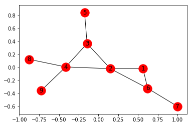
Total number of nodes: 9
Total number of edges: 10
List of all nodes: [1, 2, 3, 4, 5, 6, 7, 8, 9]
List of all edges: [(1, 2, {}), (1, 6, {}), (2, 3, {}), (2, 4, {}), (2, 6, {}), (3, 4, {}), (3, 5, {}), (4, 8, {}), (4, 9, {}), (6, 7, {})]
Degree for all nodes: {1: 2, 2: 4, 3: 3, 4: 4, 5: 1, 6: 3, 7: 1, 8: 1, 9: 1}
Total number of self-loops: 0
List of all nodes with self-loops: []
List of all nodes we can go to in a single step from node 2: [1, 3, 4, 6]
创建加权无向图 -
添加所有边的列表以及各种权重 -
import networkx as nx
G = nx.Graph()

edges = [(1, 2, 19), (1, 6, 15), (2, 3, 6), (2, 4, 10),
         (2, 6, 22), (3, 4, 51), (3, 5, 14), (4, 8, 20),
         (4, 9, 42), (6, 7, 30)]

G.add_weighted_edges_from(edges)
nx.draw_networkx(G, with_labels = True)
我们可以通过边缘列表添加边缘,需要以.txt格式保存(例如 edge_list.txt)
G = nx.read_edgelist('edge_list.txt', data =[('Weight', int)])
1 2 19
1 6 15
2 3 6
2 4 10
2 6 22
3 4 51
3 5 14
4 8 20
4 9 42
6 7 30
边缘列表也可以通过 Pandas 数据框读取 -
import pandas as pd

df = pd.read_csv('edge_list.txt', delim_whitespace = True,
                   header = None, names =['n1', 'n2', 'weight'])

G = nx.from_pandas_dataframe(df, 'n1', 'n2', edge_attr ='weight')

# The Graph diagram does not show the edge weights.
# However, we can get the weights by printing all the
# edges along with the weights by the command below
print(list(G.edges(data = True)))
输出:
[(1, 2, {'weight': 19}),
 (1, 6, {'weight': 15}),
 (2, 3, {'weight': 6}),
 (2, 4, {'weight': 10}),
 (2, 6, {'weight': 22}),
 (3, 4, {'weight': 51}),
 (3, 5, {'weight': 14}),
 (4, 8, {'weight': 20}),
 (4, 9, {'weight': 42}),
 (6, 7, {'weight': 30})]
我们现在将探索图表的不同可视化技术。
为此,我们创建了印度各个城市的数据集以及它们之间的距离,并将其保存在.txt文件edge_list.txt中。
Kolkata Mumbai 2031
Mumbai Pune 155
Mumbai Goa 571
Kolkata Delhi 1492
Kolkata Bhubaneshwar 444
Mumbai Delhi 1424
Delhi Chandigarh 243
Delhi Surat 1208
Kolkata Hyderabad 1495
Hyderabad Chennai 626
Chennai Thiruvananthapuram 773
Thiruvananthapuram Hyderabad 1299
Kolkata Varanasi 679
Delhi Varanasi 821
Mumbai Bangalore 984
Chennai Bangalore 347
Hyderabad Bangalore 575
Kolkata Guwahati 1031
现在,我们将通过以下代码制作一个图表。我们还将为所有城市添加一个节点属性,这将是每个城市的人口。
import networkx as nx

G = nx.read_weighted_edgelist('edge_list.txt', delimiter =" ")

population = {
        'Kolkata' : 4486679,
        'Delhi' : 11007835,
        'Mumbai' : 12442373,
        'Guwahati' : 957352,
        'Bangalore' : 8436675,
        'Pune' : 3124458,
        'Hyderabad' : 6809970,
        'Chennai' : 4681087,
        'Thiruvananthapuram' : 460468,
        'Bhubaneshwar' : 837737,
        'Varanasi' : 1198491,
        'Surat' : 4467797,
        'Goa' : 40017,
        'Chandigarh' : 961587
        }

# We have to set the population attribute for each of the 14 nodes
for i in list(G.nodes()):
    G.nodes[i]['population'] = population[i]

nx.draw_networkx(G, with_label = True)
# This line allows us to visualize the Graph
输出: 
但是,我们可以通过以下步骤自定义网络以直观地提供更多信息:
- 节点的大小与城市的人口成正比。
- 节点的颜色强度与节点的度数成正比。
- 边缘的宽度与边缘的权重成正比,在这种情况下,城市之间的距离。
# fixing the size of the figure
plt.figure(figsize =(10, 7))

node_color = [G.degree(v) for v in G]
# node colour is a list of degrees of nodes

node_size = [0.0005 * nx.get_node_attributes(G, 'population')[v] for v in G]
# size of node is a list of population of cities

edge_width = [0.0015 * G[u][v]['weight'] for u, v in G.edges()]
# width of edge is a list of weight of edges

nx.draw_networkx(G, node_size = node_size,
                 node_color = node_color, alpha = 0.7,
                 with_labels = True, width = edge_width,
                 edge_color ='.4', cmap = plt.cm.Blues)

plt.axis('off')
plt.tight_layout();
输出: 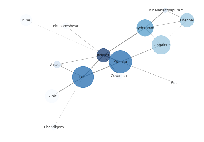
我们可以在上面的代码中看到,我们将布局类型指定为紧。您可以找到不同的布局技术并尝试其中一些,如下面的代码所示:
print("The various layout options are:")
print([x for x in nx.__dir__() if x.endswith('_layout')])
# prints out list of all different layout options

node_color = [G.degree(v) for v in G]
node_size = [0.0005 * nx.get_node_attributes(G, 'population')[v] for v in G]
edge_width = [0.0015 * G[u][v]['weight'] for u, v in G.edges()]

plt.figure(figsize =(10, 9))
pos = nx.random_layout(G)
print("Random Layout:")

# demonstrating random layout
nx.draw_networkx(G, pos, node_size = node_size,
                 node_color = node_color, alpha = 0.7,
                 with_labels = True, width = edge_width,
                 edge_color ='.4', cmap = plt.cm.Blues)


plt.figure(figsize =(10, 9))
pos = nx.circular_layout(G)
print("Circular Layout")

# demonstrating circular layout
nx.draw_networkx(G, pos, node_size = node_size,
                 node_color = node_color, alpha = 0.7,
                 with_labels = True, width = edge_width,
                 edge_color ='.4', cmap = plt.cm.Blues)
输出:
各种布局选项有: ['rescale_layout', 'random_layout', 'shell_layout', 'fruchterman_reingold_layout', 'spectral_layout', 'kamada_kawai_layout', 'spring_layout', 'circular_layout'] 随机布局: 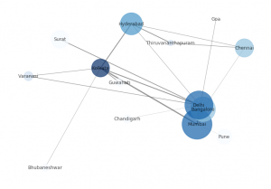 圆形布局:
圆形布局: 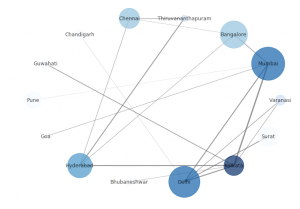
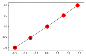
Networkx 允许我们创建路径图,即以下列方式连接多个节点的直线:
G2 = nx.path_graph(5)
nx.draw_networkx(G2, with_labels = True)
我们可以重命名节点——
G2 = nx.path_graph(5)

new = {0:"Germany", 1:"Austria", 2:"France", 3:"Poland", 4:"Italy"}
G2 = nx.relabel_nodes(G2, new)
nx.draw_networkx(G2, with_labels = True)

创建有向图 -
Networkx 允许我们使用有向图。它们的创建、添加节点、边等与此处讨论的无向图完全相同。
以下代码显示了有向图的基本操作。
import networkx as nx
G = nx.DiGraph()
G.add_edges_from([(1, 1), (1, 7), (2, 1), (2, 2), (2, 3),
                  (2, 6), (3, 5), (4, 3), (5, 4), (5, 8),
                  (5, 9), (6, 4), (7, 2), (7, 6), (8, 7)])

plt.figure(figsize =(9, 9))
nx.draw_networkx(G, with_label = True, node_color ='green')

# getting different graph attributes
print("Total number of nodes: ", int(G.number_of_nodes()))
print("Total number of edges: ", int(G.number_of_edges()))
print("List of all nodes: ", list(G.nodes()))
print("List of all edges: ", list(G.edges()))
print("In-degree for all nodes: ", dict(G.in_degree()))
print("Out degree for all nodes: ", dict(G.out_degree))

print("Total number of self-loops: ", int(G.number_of_selfloops()))
print("List of all nodes with self-loops: ",
             list(G.nodes_with_selfloops()))

print("List of all nodes we can go to in a single step from node 2: ",
                                                list(G.successors(2)))

print("List of all nodes from which we can go to node 2 in a single step: ",
                                                    list(G.predecessors(2)))
输出: 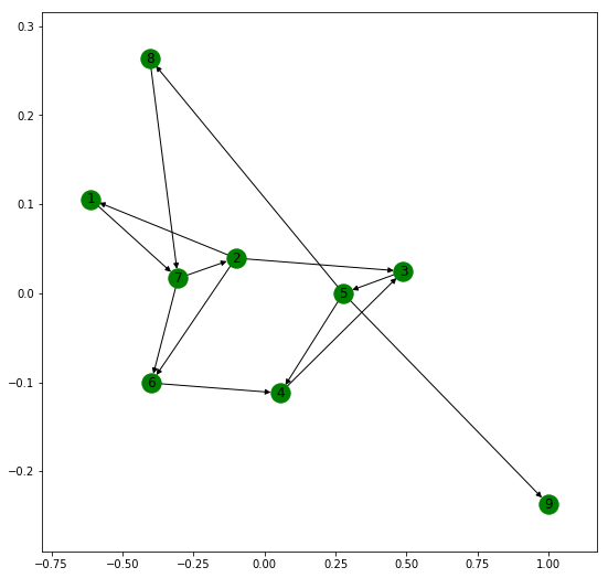
Total number of nodes: 9
Total number of edges: 15
List of all nodes: [1, 2, 3, 4, 5, 6, 7, 8, 9]
List of all edges: [(1, 1), (1, 7), (2, 1), (2, 2), (2, 3), (2, 6), (3, 5), (4, 3), (5, 8), (5, 9), (5, 4), (6, 4), (7, 2), (7, 6), (8, 7)]
In-degree for all nodes: {1: 2, 2: 2, 3: 2, 4: 2, 5: 1, 6: 2, 7: 2, 8: 1, 9: 1}
Out degree for all nodes: {1: 2, 2: 4, 3: 1, 4: 1, 5: 3, 6: 1, 7: 2, 8: 1, 9: 0}
Total number of self-loops: 2
List of all nodes with self-loops: [1, 2]
List of all nodes we can go to in a single step from node 2: [1, 2, 3, 6]
List of all nodes from which we can go to node 2 in a single step: [2, 7]
现在,我们将展示 MultiGraph 的基本操作。 Networkx 允许我们创建有向和无向多图。多图是多条平行边可以连接相同节点的图。
例如,让我们创建一个由 10 个人组成的网络,A、B、C、D、E、F、G、H、I 和 J。他们之间有四种不同的关系,即朋友、同事、家人和邻居。两个人之间的关系并不局限于一种关系。
但是 Networkx 中 Multigraph 的可视化并不清楚。它无法分别显示多个边缘并且这些边缘重叠。
import networkx as nx
import matplotlib.pyplot as plt

G = nx.MultiGraph()
relations = [('A', 'B', 'neighbour'), ('A', 'B', 'friend'), ('B', 'C', 'coworker'),
             ('C', 'F', 'coworker'), ('C', 'F', 'friend'), ('F', 'G', 'coworker'),
             ('F', 'G', 'family'), ('C', 'E', 'friend'), ('E', 'D', 'family'),
             ('E', 'I', 'coworker'), ('E', 'I', 'neighbour'), ('I', 'J', 'coworker'),
             ('E', 'J', 'friend'), ('E', 'H', 'coworker')]

for i in relations:
    G.add_edge(i[0], i[1], relation = i[2])

plt.figure(figsize =(9, 9))
nx.draw_networkx(G, with_label = True)

# getting various graph properties
print("Total number of nodes: ", int(G.number_of_nodes()))
print("Total number of edges: ", int(G.number_of_edges()))
print("List of all nodes: ", list(G.nodes()))
print("List of all edges: ", list(G.edges(data = True)))
print("Degree for all nodes: ", dict(G.degree()))
print("Total number of self-loops: ", int(G.number_of_selfloops()))
print("List of all nodes with self-loops: ", list(G.nodes_with_selfloops()))
print("List of all nodes we can go to in a single step from node E: ",
                                               list(G.neighbors('E")))
输出: 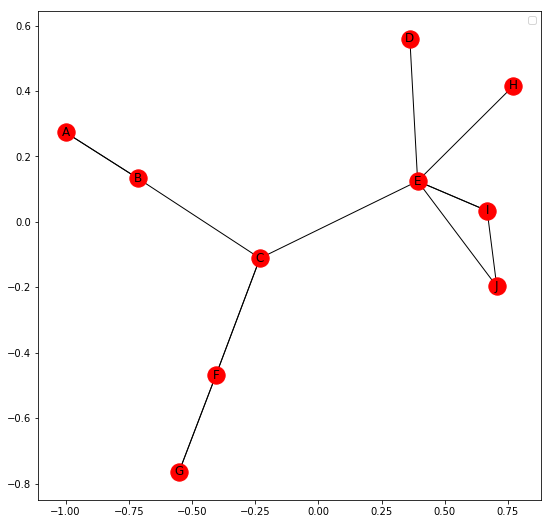
Total number of nodes: 10
Total number of edges: 14
List of all nodes: [‘E’, ‘I’, ‘D’, ‘B’, ‘C’, ‘F’, ‘H’, ‘A’, ‘J’, ‘G’]
List of all edges: [(‘E’, ‘I’, {‘relation’: ‘coworker’}), (‘E’, ‘I’, {‘relation’: ‘neighbour’}), (‘E’, ‘H’, {‘relation’: ‘coworker’}), (‘E’, ‘J’, {‘relation’: ‘friend’}), (‘E’, ‘C’, {‘relation’: ‘friend’}), (‘E’, ‘D’, {‘relation’: ‘family’}), (‘I’, ‘J’, {‘relation’: ‘coworker’}), (‘B’, ‘A’, {‘relation’: ‘neighbour’}), (‘B’, ‘A’, {‘relation’: ‘friend’}), (‘B’, ‘C’, {‘relation’: ‘coworker’}), (‘C’, ‘F’, {‘relation’: ‘coworker’}), (‘C’, ‘F’, {‘relation’: ‘friend’}), (‘F’, ‘G’, {‘relation’: ‘coworker’}), (‘F’, ‘G’, {‘relation’: ‘family’})]
Degree for all nodes: {‘E’: 6, ‘I’: 3, ‘B’: 3, ‘D’: 1, ‘F’: 4, ‘A’: 2, ‘G’: 2, ‘H’: 1, ‘J’: 2, ‘C’: 4}
Total number of self-loops: 0
List of all nodes with self-loops: []
List of all nodes we can go to in a single step from node E: [‘I’, ‘H’, ‘J’, ‘C’, ‘D’]
类似地,可以使用创建多向图
G = nx.MultiDiGraph()
在评论中写代码?请使用 ide.geeksforgeeks.org,生成链接并在此处分享链接。