在Python中解决线性回归
线性回归是对因变量与一个或多个自变量之间的关系进行建模的常用方法。使用从数据估计的参数开发线性模型。线性回归在预测和预测中很有用,其中预测模型适合观察到的值数据集以确定响应。线性回归模型通常使用最小二乘法拟合,其目标是最小化误差。
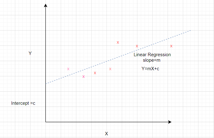
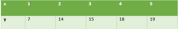
考虑一个数据集,其中独立属性由 x 表示,从属属性由 y 表示。
已知直线方程为y = mx + b ,其中 m 是斜率,b 是截距。
为了准备给定数据集的简单回归模型,我们需要计算最适合数据点的直线的斜率和截距。
如何计算斜率和截距?
计算斜率和截距的数学公式如下
Slope = Sxy/Sxx
where Sxy and Sxx are sample covariance and sample variance respectively.

Intercept = ymean – slope* xmean
让我们使用这些关系来确定上述数据集的线性回归。为此,我们计算 x均值、 y均值、 S xy 、 S xx ,如表中所示。

根据上述公式,
斜率 = 28/10 = 2.8
截距 = 14.6 – 2.8 * 3 = 6.2
所以,
The desired equation of the regression model is y = 2.8 x + 6.2我们将使用这些值来预测给定 x 值的 y 值。可以通过计算均方根误差和R 2值来分析模型的性能。
计算如下所示。 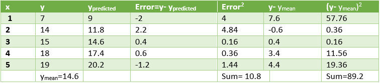
Squared Error=10.8 这意味着均方误差 = 3.28
测定系数 (R 2 ) = 1- 10.8 / 89.2 = 0.878
Low value of error and high value of R2 signify that the
linear regression fits data well
让我们看看这个数据集的线性回归的Python实现。
代码 1:导入所有必要的库。
import numpy as np
import matplotlib.pyplot as plt

from sklearn.linear_model import LinearRegression
from sklearn.metrics import mean_squared_error, r2_score
import statsmodels.api as sm
代码 2:生成数据。计算 x mean , y mean , Sxx, Sxy 求回归线的斜率和截距值。
x = np.array([1,2,3,4,5])
y = np.array([7,14,15,18,19])
n = np.size(x)

x_mean = np.mean(x)
y_mean = np.mean(y)
x_mean,y_mean

Sxy = np.sum(x*y)- n*x_mean*y_mean
Sxx = np.sum(x*x)-n*x_mean*x_mean

b1 = Sxy/Sxx
b0 = y_mean-b1*x_mean
print('slope b1 is', b1)
print('intercept b0 is', b0)

plt.scatter(x,y)
plt.xlabel('Independent variable X')
plt.ylabel('Dependent variable y')
输出:
slope b1 is 2.8
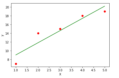
intercept b0 is 6.200000000000001代码 3:绘制给定的数据点并拟合回归线。
y_pred = b1 * x + b0

plt.scatter(x, y, color = 'red')
plt.plot(x, y_pred, color = 'green')
plt.xlabel('X')
plt.ylabel('y')
代码 4:通过计算均方误差和 R 2来分析模型的性能
error = y - y_pred
se = np.sum(error**2)
print('squared error is', se)

mse = se/n
print('mean squared error is', mse)

rmse = np.sqrt(mse)
print('root mean square error is', rmse)

SSt = np.sum((y - y_mean)**2)
R2 = 1- (se/SSt)
print('R square is', R2)
输出:
squared error is 10.800000000000004
mean squared error is 2.160000000000001
root mean square error is 1.4696938456699071
R square is 0.8789237668161435
代码5:使用scikit库确认上述步骤。
x = x.reshape(-1,1)
regression_model = LinearRegression()

# Fit the data(train the model)
regression_model.fit(x, y)

# Predict
y_predicted = regression_model.predict(x)

# model evaluation
mse=mean_squared_error(y,y_predicted)

rmse = np.sqrt(mean_squared_error(y, y_predicted))
r2 = r2_score(y, y_predicted)

# printing values
print('Slope:' ,regression_model.coef_)
print('Intercept:', regression_model.intercept_)
print('MSE:',mse)
print('Root mean squared error: ', rmse)
print('R2 score: ', r2)
输出:
Slope: [2.8]
Intercept: 6.199999999999999
MSE: 2.160000000000001
Root mean squared error:  1.4696938456699071
R2 score: 0.8789237668161435结论:本文有助于理解简单回归背后的数学原理,并使用Python实现它。