TensorFlow 2.0

TensorFlow是一个广受欢迎的开源平台，用于开发和集成大规模AI和深度学习模型，最近已更新为TensorFlow 2.0的更新形式。这极大地提升了TensorFlow社区创建的原本功能丰富的ML生态系统中的功能。

什么是开源，它如何使TensorFlow如此成功?
开源是指人们(主要是开发人员)可以修改，共享和集成的东西，因为所有原始设计功能都向所有人开放。这使得特定软件，产品的扩展非常容易，有效且耗时极短。此功能使TensorFlow的原始创建者(即Google)可以轻松地将其移植到市场上可用的每个平台中，包括Web，移动，物联网，嵌入式系统，边缘计算，并包括对其他各种语言的支持，例如JavaScript，Node.js， F＃，C++，C＃，React.js，Go，Julia，Rust，Android，Swift，Kotlin等。
随之而来的是对运行大型机器学习代码的硬件加速的支持。这些包括CUDA(用于在GPU上运行ML代码的库)，TPU(张量处理单元-由Google提供的定制硬件，专门设计和开发用于使用TensorFlow处理张量的多机器配置)，GPU，GPGPU，基于云的TPU，ASIC(专用集成电路)FPGA(现场可编程门阵列-这些专用于定制的可编程硬件)。这还包括新增加的功能，例如NVIDIA的Jetson TX2和英特尔的Movidius芯片。
现在回到新的且功能丰富的TensorFlow2.0：
这是更改的图形实现：

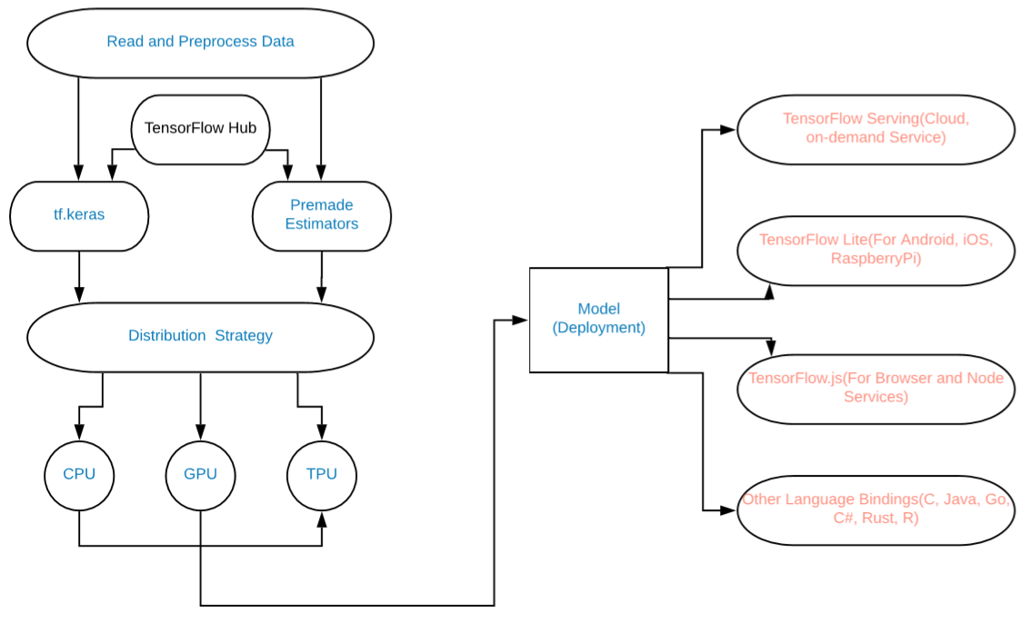
模型图

添加的内容包括：

现在，除了Keras之外，其他主要API均已使用：Keras的流体层现在集成在原始TensorFlow代码之上，从而使其变得简单易用。这将有助于在机器学习和AI领域带来很多进步和生产力。

急切的命令行：这个简单的命令行可以帮助我们立即执行操作，而无需使用Session.run命令。

简化和集成的工作流程：

1. 使用tf.data进行数据加载(或NumPy)。
2. 使用Keras进行模型构建(我们也可以使用任何预制的Estimators)。
3. 使用tf。 DAG图形执行函数或使用预先执行功能。
4. 将分布策略用于高性能计算和深度学习模型。 (用于TPU，GPU等)。
5. TF 2.0将Saved Model标准化为TensorFlow图的序列化版本，适用于Mobile，JavaScript，TensorBoard，TensorHub等各种平台。

支持TensorFlow Lite和TensorFlow边缘计算：这将有助于开发人员为终端设备提供有效的机器学习和AI服务。这将需要非常少的计算能力以及更快的模型实现和最终用户

使用TensorFlow.js的Web应用程序和Node.js的新扩展，用于基于AI的新的交互式网站和应用程序。

适用于Android的TensorFlow优化。

TensorFlow集成，用于基于Swift和IOS的应用程序。

支持即将发布的最迫切的WebGPU Chrome RFC提案。

统一编程范例(有向无环图/功能和堆栈/顺序)。

TensorFlow AIY(您自己的人工智能)支持。

将tf.contrib集成到单独的存储库中。

改进的TPU和TPU支持以及分布式计算支持以及对v3的支持。

改进的用于并行计算的HPC集成。

开发，支持和研究的社区整合。

将tf.contrib最佳程序包实现集成到核心程序包中。

特定于域的社区支持。

对模型验证和重用的额外支持。

TensorFlow Hub上提供了端到端ML管道和产品。

最后，我们现在可以轻松地在TensorFlow2.0上为最终用户轻松构建大型ML和深度学习模型，并大规模实施它们。

例子：
训练神经网络对MNSIT数据进行分类

# Write Python3 code here
import tensorflow as tf
  
"""The Fashion MNIST data is available directly in the tf.keras
 datasets API. You load it like this:"""
  
mnist = tf.keras.datasets.fashion_mnist
  
"""Calling load_data on this object will give you two sets of two
 lists, these will be the training and testing values for the graphics
 that contain the clothing items and their labels."""
  
(training_images, training_labels), (test_images, test_labels) = mnist.load_data()
"""You'll notice that all of the values in the number are between 0 and 255. 
If we are training a neural network, for various reasons it's easier if we
treat all values as between 0 and 1, a process called '**normalizing**'...and
fortunately in Python it's easy to normalize a list like this without looping.
So, perform it like - """
  
training_images  = training_images / 255.0
test_images = test_images / 255.0
  
"""Now you might be wondering why there are 2 sets...training and testing
-- remember we spoke about this in the intro? The idea is to have 1 set of
data for training, and then another set of data...that the model hasn't yet
seen...to see how good it would be at classifying values. After all, when
you're done, you're going to want to try it out with data that it hadn't 
previously seen!
  
Let's now design the model. There are quite a few new concepts here, 
but don't worry, you'll get the hang of them.
"""
  
model = tf.keras.models.Sequential([tf.keras.layers.Flatten(), 
                                    tf.keras.layers.Dense(
                                            128, activation=tf.nn.relu), 
                                    tf.keras.layers.Dense(
                                            10, activation=tf.nn.softmax)])
  
"""**Sequential**: That defines a SEQUENCE of layers in the neural network
  
**Flatten**: Remember earlier where our images were a square when
you printed them out? Flatten just takes that square and turns it
into a 1-dimensional set.
  
**Dense**: Adds a layer of neurons
  
Each layer of neurons needs an **activation function** to tell them what to
do. There are lots of options, but just use these for now. 
  
**Relu** effectively means "If X>0 return X, else return 0" -- so what it does
 it only passes values 0 or greater to the next layer in the network.
  
**Softmax** takes a set of values, and effectively picks the biggest one, so,
 for example, if the output of the last layer looks like [0.1, 0.1, 0.05, 0.1,
 9.5, 0.1, 0.05, 0.05, 0.05], it saves you from fishing through it looking for
 the biggest value, and turns it into [0,0,0,0,1,0,0,0,0] -- 
 The goal is to save a lot of coding!
  
The next thing to do, now the model is defined, is to actually build it.
You do this by compiling it with an optimizer and loss function as before -- 
and then you train it by calling **model.fit ** asking it to fit your training
data to your training labels -- i.e. have it figure out the relationship between
the training data and its actual labels, so in future, if you have data that
looks like the training data, then it can make a prediction for what that data
would look like.
"""
  
model.compile(optimizer = tf.keras.optimizers.Adam(),
              loss = 'sparse_categorical_crossentropy',
              metrics=['accuracy'])
  
model.fit(training_images, training_labels, epochs=5)
  
"""Once it's done training -- you should see an accuracy value at the end of the
final epoch. It might look something like 0.9098. This tells you that your
neural network is about 91% accurate in classifying the training data. I.E.,
it figured out a pattern match between the image and the labels that worked
91% of the time. Not great, but not bad considering it was only trained for 5
epochs and done quite quickly.
  
But how would it work with unseen data? That's why we have the test images. We 
can call model.evaluate, and pass in the two sets, and it will report back the
loss for each. Let's give it a try:
"""
  
model.evaluate(test_images, test_labels)
  
""" For me, that returned an accuracy of about .8838, which means it was 
about 88% accurate. As expected it probably would not do as well with *unseen*
data as it did with data it was trained on!  
 """

输出：

Expected Accuracy 88-91%

渴望执行：

import tensorflow as tf
import tensorflow.contrib.eager as tfe
   
tfe.enable_eager_execution()
   
x = [[2.]]
m = tf.matmul(x, x)
   
print(m)

输出 ：

tf.Tensor([[4.]], shape=(1, 1), dtype=float32)