使用分类进行肿瘤检测——机器学习和Python

在本文中，我们将通过Python语言制作一个项目，该项目也将使用一些机器学习算法。这将是一个令人兴奋的项目，因为在这个项目之后，您将了解通过脚本语言使用 AI 和 ML 的概念。本项目将使用以下库/包：

• numpy ：它是一个用于科学计算的Python库。它包含一个强大的数组对象、用于与其他语言代码（即 C/C++ 和 Fortran 代码）集成的数学和统计工具。
• pandas ：它是一个Python包，提供快速、灵活和富有表现力的数据结构，旨在轻松直观地处理“关系”或“标记”数据。
• matplotlib ： Matplotlib 可能是Python编程语言的绘图库，它生成 2D 绘图以呈现可视化并有助于探索信息集。 matplotlib.pyplot 可以是一组命令样式函数，使 matplotlib 像 MATLAB 一样工作。
• 塞尔伯恩： 。 Seaborn 是一个建立在 matplotlib 之上的开源Python库。它用于数据可视化和探索性数据分析。 Seaborn 可以轻松处理数据框和 Pandas 库。

Python3

# Checking for any warning
import warnings
warnings.filterwarnings('ignore')

在这一步之后，我们将安装一些依赖项：依赖项是项目所需的所有软件组件，以便它按预期工作并避免运行时错误。我们将需要numpy、pandas、matplotlib 和 seaborn 库/依赖项。由于我们需要一个 CSV 文件来执行操作，因此对于这个项目，我们将使用一个包含肿瘤（脑疾病）数据的 CSV 文件。所以在这个项目中，我们终于能够预测一个受试者（候选人）是否有可能患上肿瘤？

第 1 步：预处理数据：

蟒蛇3

# Importing dependencies
import numpy as np
import pandas as pd
import matplotlib.pyplot as plt
import seaborn as sns
 
# Including & Reading the CSV file:
df = pd.read_csv("https://raw.githubusercontent.com/ingledarshan/AIML-B2/main/data.csv")

现在我们将检查 CSV 文件是否已成功读取？所以我们将使用head 方法： head() 方法用于返回数据框或系列的前 n（默认为 5）行。

蟒蛇3

df.head()

蟒蛇3

# Check the names of all columns
df.columns

所以这个命令将获取列的标题名称。输出将是这样的：

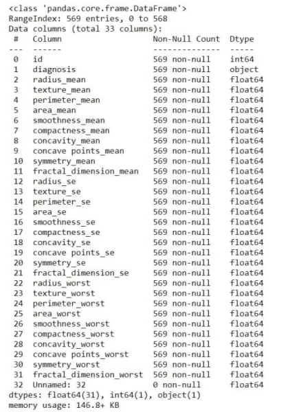
现在为了通过快速概览数据集来简要了解数据集，我们将使用info() 方法。这种方法很好地处理了数据集的探索性分析。

蟒蛇3

df.info()

上述命令的输出：

在 CSV 文件中，可能有一些空白字段可能会损害项目（即它们会妨碍预测）。

蟒蛇3

df['Unnamed: 32']

输出：

现在我们已经成功地找到了数据集中的空位，所以现在我们将删除它们。

蟒蛇3

df = df.drop("Unnamed: 32", axis=1)
 
# to check whether those values are
# deletd or not:
df.head()
 
# also check the columns after this
# process:
df.columns
 
df.drop('id', axis=1, inplace=True)
# we can do this also: df = df.drop('id', axis=1)
 
# To see the change, again go through
# the columns
df.columns

现在我们将在type() 方法的帮助下检查列的类类型。它返回作为参数传递的参数（对象）的类类型。

蟒蛇3

type(df.columns)

输出：

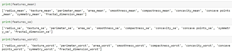
pandas.core.indexes.base.Index

我们将需要按列对数据进行遍历和排序，因此我们将这些列保存在一个变量中。

蟒蛇3

l = list(df.columns)
print(l)

现在我们将访问具有不同起点的数据。假设我们将在名为features_mean的变量中对从 1 到 11 的列进行分类，依此类推。

蟒蛇3

features_mean = l[1:11]
 
features_se = l[11:21]
 
features_worst = l[21:]

蟒蛇3

df.head (2)

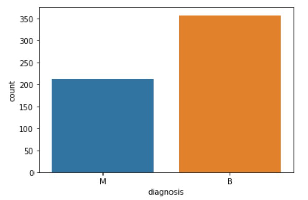
在 CSV 文件的“诊断”栏中，有两个选项，一个是M = 恶性和 B = 开始，它基本上告诉了肿瘤的阶段。但同样我们将从代码中验证。

蟒蛇3

# To check what value does the Diagnosis field have
df['diagnosis'].unique()
# M stands for Malignant, B stands for Begin

输出：

array(['M', 'B'], dtype=object)

因此它验证诊断字段中只有两个值。

现在为了清楚地了解有多少病例患有恶性肿瘤以及哪些人处于开始阶段，我们将使用 countplot() 方法。

蟒蛇3

sns.countplot(df['diagnosis'], label="Count",);

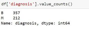
如果我们不必查看值的图形，那么我可以使用一个函数来返回出现的数值。

现在我们将能够使用 shape() 方法。 Shape 返回数组的形式。形式可以是整数元组。这些数字表示相应数组维度的长度。换句话说：数组的“形状”可能是一个元组，每个轴（维度）的元素数。例如，该形式足以满足 (6, 3) 的要求，即我们有 6 行和 3 列。

蟒蛇3

df.shape

输出：

(539, 31)

这意味着在数据集中有 539 行和 31 列。

到目前为止，我们已经准备好要处理的数据集，所以我们将能够使用 describe() 方法来查看知识框架的一些基本统计细节，如百分位数、均值、标准差等或一系列数值。

蟒蛇3

# Summary of all numeric values
df.decsbibe()

毕竟，这个东西，我们将使用 corr() 方法来查找不同字段之间的相关性。 Corr()用于查找数据框中所有列的成对相关性。任何 nan 值都会被自动排除。对于数据框中的任何非数字数据类型列，它都会被忽略。

蟒蛇3

# Correlation Plot
corr = df.corr()
corr

此命令将提供 30 行 * 30 列的表，其中包含诸如radius_mean、texture_se等行。

命令 corr.shape() 将返回 (30, 30)。下一步是通过热图绘制统计数据。热图甚至可以是信息的二维图形表示，其中包含在矩阵中的各个值以颜色表示。 seaborn 包允许创建带注释的热图，可以根据创建者的要求使用 Matplotlib 工具对其进行一些更改。

蟒蛇3

# making a heatmap
plt.figure(figsize=(14, 14))
sns.heatmap(corr)

我们将再次检查 CSV 数据集，以确保列正常且未受操作影响。

蟒蛇3

df.head()

这将返回一个表，通过该表可以确保数据集是否排序良好。在接下来的几个命令中，我们将分离数据。

蟒蛇3

df['diagnosis'] = df['diagnosis'].map({'M': 1, 'B': 0})
df.head()
 
df['diagnosis'].unique()
 
X = df.drop('diagnosis', axis=1)
X.head()
 
y = df['diagnosis']
y.head()

注意：由于我们已经准备了一个可以与任何机器学习模型一起使用的预测模型，所以现在我们将使用每个机器学习算法向您展示预测模型的输出。

步骤 2：测试检查或训练数据集

• 使用逻辑回归模型：

蟒蛇3

# divide the dataset into train and test set
from sklearn.preprocessing import StandardScaler
from sklearn.model_selection import train_test_split
X_train, X_test, y_train, y_test = train_test_split(X, y, test_size=0.3)
 
df.shape
# o/p: (569, 31)
 
X_train.shape
# o/p: (398, 30)
 
X_test.shape
# o/p: (171, 30)
 
y_train.shape
# o/p: (398,)
 
y_test.shape
# o/p: (171,)
 
X_train.head(1)
# will return the top 5 rows (if exists)
 
ss = StandardScaler()
X_train = ss.fit_transform(X_train)
X_test = ss.transform(X_test)
 
X_train

输出：

在完成模型的基本训练后，我们可以使用其中一种机器学习模型进行测试。因此，我们将使用逻辑回归、决策树分类器、随机森林分类器和 SVM来测试这一点。

蟒蛇3

# apply Logistic Regression
 
from sklearn.linear_model import LogisticRegression
lr = LogisticRegression()
lr.fit(X_train, y_train)
 
# implemented our model through logistic regression
y_pred = lr.predict(X_test)
y_pred
 
# array containing the actual output
y_test

输出：

从数学上检查模型预测正确值的程度：

蟒蛇3

from sklearn.metrics import accuracy_score
print(accuracy_score(y_test, y_pred))

输出：

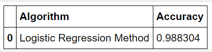
0.9883040935672515

现在让我们以表格的形式将结果框起来。

蟒蛇3

tempResults = pd.DataFrame({'Algorithm':['Logistic Regression Method'], 'Accuracy':[lr_acc]})
results = pd.concat( [results, tempResults] )
results = results[['Algorithm','Accuracy']]
results

输出：

• 使用决策树模型：

蟒蛇3

# apply Decision Tree Classifier
from sklearn.metrics import accuracy_score
from sklearn.tree import DecisionTreeClassifier
dtc = DecisionTreeClassifier()
dtc.fit(X_train, y_train)
 
y_pred = dtc.predict(X_test)
y_pred
 
print(accuracy_score(y_test, y_pred))
 
# Tabulating the results
tempResults = pd.DataFrame({'Algorithm': ['Decision tree Classifier Method'],
                            'Accuracy': [dtc_acc]})
results = pd.concat([results, tempResults])
results = results[['Algorithm', 'Accuracy']]
results

输出：

• 使用随机森林模型：

蟒蛇3

# apply Random Forest Classifier
from sklearn.metrics import accuracy_score
from sklearn.ensemble import RandomForestClassifier
rfc = RandomForestClassifier()
rfc.fit(X_train, y_train)
 
y_pred = rfc.predict(X_test)
y_pred
 
print(accuracy_score(y_test, y_pred))
 
# tabulating the results
tempResults = pd.DataFrame({'Algorithm': ['Random Forest Classifier Method'],
                            'Accuracy': [rfc_acc]})
 
results = pd.concat([results, tempResults])
results = results[['Algorithm', 'Accuracy']]
results

输出：

• 使用支持向量机：

蟒蛇3

# apply Support Vector Machine
from sklearn import svm
svc = svm.SVC()
svc.fit(X_train,y_train
         
y_pred = svc.predict(X_test)
y_pred
         
from sklearn.metrics import accuracy_score
print(accuracy_score(y_test, y_pred))

输出：

所以现在我们可以通过这个表检查哪个模型有效地产生了更多的正确预测：

蟒蛇3

# Tabulating the results
tempResults = pd.DataFrame({'Algorithm': ['Support Vector Classifier Method'],
                            'Accuracy': [svc_acc]})
results = pd.concat([results, tempResults])
results = results[['Algorithm', 'Accuracy']]
results

输出：

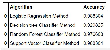
在检查了上述机器学习算法的准确性后，我可以得出结论，如果输入相同的数据集，这些算法每次都会给出相同的输出。我也可以说，即使数据集发生变化，这些算法也主要提供相同的预测精度输出。

从上表中，我们可以得出结论，通过 SVM 模型和逻辑回归模型是最适合我的项目的模型。