科学 |曲线拟合

给定一个由一组点组成的数据集，找到表示数据的最佳拟合。
我们经常有一个由遵循一般路径的数据组成的数据集，但每个数据都有一个标准偏差，这使得它们分散在最佳拟合线上。我们可以使用 curve-fit()函数得到一条线。
使用 SciPy：
Scipy 是Python的科学计算模块，在许多著名的数学函数上提供了内置函数。 scipy.optimize 包为我们提供了多种优化程序。在 iPython 控制台中键入以下内容可以找到 Optimize 的所有功能的详细列表：

help(scipy.optimize)

其中最常用的是最小二乘法、曲线拟合、多元标量函数的最小化等。
曲线拟合示例 –
输入 ：

输出 ：

输入 ：

输出 ：

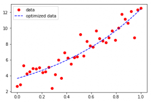
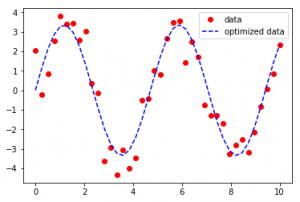
从输入中可以看出，数据集似乎分散在第一种情况下的正弦函数和第二种情况下的指数函数中，Curve-Fit 赋予函数合法性并确定系数以提供最佳拟合线。显示第一个示例生成的代码 -

Python3

import numpy as np
 
# curve-fit() function imported from scipy
from scipy.optimize import curve_fit
 
from matplotlib import pyplot as plt
 
# numpy.linspace with the given arguments
# produce an array of 40 numbers between 0
# and 10, both inclusive
x = np.linspace(0, 10, num = 40)
 
 
# y is another array which stores 3.45 times
# the sine of (values in x) * 1.334.
# The random.normal() draws random sample
# from normal (Gaussian) distribution to make
# them scatter across the base line
y = 3.45 * np.sin(1.334 * x) + np.random.normal(size = 40)
 
# Test function with coefficients as parameters
def test(x, a, b):
    return a * np.sin(b * x)
 
# curve_fit() function takes the test-function
# x-data and y-data as argument and returns
# the coefficients a and b in param and
# the estimated covariance of param in param_cov
param, param_cov = curve_fit(test, x, y)
 
 
print("Sine function coefficients:")
print(param)
print("Covariance of coefficients:")
print(param_cov)
 
# ans stores the new y-data according to
# the coefficients given by curve-fit() function
ans = (param[0]*(np.sin(param[1]*x)))
 
'''Below 4 lines can be un-commented for plotting results
using matplotlib as shown in the first example. '''
 
# plt.plot(x, y, 'o', color ='red', label ="data")
# plt.plot(x, ans, '--', color ='blue', label ="optimized data")
# plt.legend()
# plt.show()

输出：

Sine function coefficients:
[ 3.66474998  1.32876756]
Covariance of coefficients:
[[  5.43766857e-02  -3.69114170e-05]
 [ -3.69114170e-05   1.02824503e-04]]

第二个示例可以通过使用如下所示的 numpy 指数函数来实现：

Python3

x = np.linspace(0, 1, num = 40)
 
y = 3.45 * np.exp(1.334 * x) + np.random.normal(size = 40)
 
def test(x, a, b):
    return a*np.exp(b*x)
 
param, param_cov = curve_fit(test, x, y)

但是，如果系数太大，曲线会变平并且无法提供最佳拟合。下面的代码解释了这个事实：

Python3

import numpy as np
from scipy.optimize import curve_fit
 
from matplotlib import pyplot as plt
 
x = np.linspace(0, 10, num = 40)
 
# The coefficients are much bigger.
y = 10.45 * np.sin(5.334 * x) + np.random.normal(size = 40)
 
def test(x, a, b):
    return a * np.sin(b * x)
 
param, param_cov = curve_fit(test, x, y)
 
print("Sine function coefficients:")
print(param)
print("Covariance of coefficients:")
print(param_cov)
 
ans = (param[0]*(np.sin(param[1]*x)))
 
plt.plot(x, y, 'o', color ='red', label ="data")
plt.plot(x, ans, '--', color ='blue', label ="optimized data")
plt.legend()
plt.show()

输出：

Sine funcion coefficients:
[ 0.70867169  0.7346216 ]
Covariance of coefficients:
[[ 2.87320136 -0.05245869]
 [-0.05245869  0.14094361]]

蓝色虚线无疑是与数据集所有点的最佳优化距离的线，但它未能提供最佳拟合的正弦函数。
曲线拟合不应与回归相混淆。它们都涉及用函数逼近数据。但是曲线拟合的目标是获取数据集的值，通过这些值，一组给定的解释变量实际上可以描述另一个变量。回归是曲线拟合的一种特殊情况，但在这里您不需要以最佳方式拟合训练数据的曲线（这可能会导致过度拟合），而是需要能够泛化学习并因此预测新点的模型有效率的。