KMeans 中 k 最优值的肘部方法

先决条件： K-Means 聚类
任何无监督算法的一个基本步骤是确定可以将数据聚类到的最佳聚类数。肘部方法是确定此最佳 k 值的最流行的方法之一。
我们现在使用Python的Sklearn库来演示使用 K-Means 聚类技术的给定方法。
第 1 步：导入所需的库

Python3

from sklearn.cluster import KMeans
from sklearn import metrics
from scipy.spatial.distance import cdist
import numpy as np
import matplotlib.pyplot as plt

第 2 步：创建和可视化数据

Python3

# Creating the data
x1 = np.array([3, 1, 1, 2, 1, 6, 6, 6, 5, 6, 7, 8, 9, 8, 9, 9, 8])
x2 = np.array([5, 4, 5, 6, 5, 8, 6, 7, 6, 7, 1, 2, 1, 2, 3, 2, 3])
X = np.array(list(zip(x1, x2))).reshape(len(x1), 2)
 
# Visualizing the data
plt.plot()
plt.xlim([0, 10])
plt.ylim([0, 10])
plt.title('Dataset')
plt.scatter(x1, x2)
plt.show()

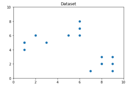
从上面的可视化我们可以看出，最优的聚类数应该在 3 左右。但是仅仅可视化数据并不能总是给出正确的答案。因此，我们演示以下步骤。
我们现在定义以下内容：-

1. 失真：计算为到各个集群的集群中心的平方距离的平均值。通常，使用欧几里得距离度量。
2. 惯性：它是样本到它们最近的聚类中心的距离平方和。

我们将 k 的值从 1 迭代到 9 并计算每个 k 值的失真值，并计算给定范围内每个 k 值的失真和惯性。
步骤 3：建立聚类模型并计算失真和惯性的值：

Python3

distortions = []
inertias = []
mapping1 = {}
mapping2 = {}
K = range(1, 10)
 
for k in K:
    # Building and fitting the model
    kmeanModel = KMeans(n_clusters=k).fit(X)
    kmeanModel.fit(X)
 
    distortions.append(sum(np.min(cdist(X, kmeanModel.cluster_centers_,
                                        'euclidean'), axis=1)) / X.shape[0])
    inertias.append(kmeanModel.inertia_)
 
    mapping1[k] = sum(np.min(cdist(X, kmeanModel.cluster_centers_,
                                   'euclidean'), axis=1)) / X.shape[0]
    mapping2[k] = kmeanModel.inertia_

第 4 步：制表和可视化结果
a)使用不同的失真值：

Python3

for key, val in mapping1.items():
    print(f'{key} : {val}')

Python3

plt.plot(K, distortions, 'bx-')
plt.xlabel('Values of K')
plt.ylabel('Distortion')
plt.title('The Elbow Method using Distortion')
plt.show()

b)使用不同的惯量值：

Python3

for key, val in mapping2.items():
    print(f'{key} : {val}')

Python3

plt.plot(K, inertias, 'bx-')
plt.xlabel('Values of K')
plt.ylabel('Inertia')
plt.title('The Elbow Method using Inertia')
plt.show()

为了确定最佳聚类数，我们必须选择“肘部”处的 k 值，即在该点之后失真/惯性开始以线性方式减小。因此，对于给定的数据，我们得出结论，数据的最佳聚类数是3 。
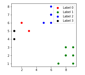
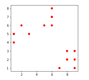
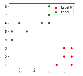
不同k值的聚类数据点：-
1. k = 1

2. k = 2

3. k = 3

4. k = 4