📌 相关文章
- TensorFlow中的多层感知器(1)
- TensorFlow-单层感知器
- TensorFlow中的单层感知器
- TensorFlow-单层感知器(1)
- TensorFlow中的单层感知器(1)
- TensorFlow-多层感知器学习(1)
- TensorFlow-多层感知器学习
- Tensorflow 中的多层感知器学习
- Tensorflow 中的多层感知器学习(1)
- PyTorch感知器(1)
- PyTorch感知器
- 如何隐藏 tensorflow 警告 (1)
- 非逻辑门感知器算法的实现(1)
- 非逻辑门感知器算法的实现
- TensorFlow 2.0(1)
- TensorFlow 2.0
- TensorFlow 2.0(1)
- TensorFlow 2.0
- 如何隐藏 tensorflow 警告 - 无论代码示例
- 具有3位二进制输入的逻辑门的感知器算法(1)
- 具有3位二进制输入的逻辑门的感知器算法
- 2位二进制输入或逻辑门感知器算法的实现(1)
- 2位二进制输入与逻辑门感知器算法的实现(1)
- 2位二进制输入或逻辑门感知器算法的实现
- 2位二进制输入与逻辑门感知器算法的实现
- 带有 Keras 的多层感知器 带有 Keras 的多层感知器 (1)
- tensorflow - Python (1)
- 带有 Keras 的多层感知器 带有 Keras 的多层感知器 - 无论代码示例
- TensorFlow-Perceptron的隐藏层(1)
📜 TensorFlow中的隐藏层感知器
📅 最后修改于: 2021-01-11 10:32:03 🧑 作者: Mango
TensorFlow中的隐藏层感知器
隐藏层是人工神经网络,位于输入层和输出层之间。人工神经元接受一组加权输入并通过激活函数产生输出。它是近乎神经的一部分,工程师可以在其中模拟人脑中正在进行的活动的类型。
隐藏的神经网络是通过某些技术建立的。在许多情况下,加权输入是随机分配的。另一方面,可以通过称为反向传播的过程对它们进行微调和校准。
感知器隐藏层中的人工神经元在大脑中充当生物神经元,它吸收其概率输入信号并对其进行处理。并将其转换为对应于生物神经元轴突的输出。
输入层之后的层称为隐藏层,因为它们直接解析为输入。最简单的网络结构是在隐藏层中具有一个直接输出值的单个神经元。
深度学习可以指的是我们的神经网络中有许多隐藏层。它们之所以很深,是因为从历史上讲它们训练起来会非常缓慢,但是使用现代技术和硬件准备可能要花费几秒钟或几分钟。
单个隐藏层将构建一个简单的网络。
感知器的隐藏层的代码如下所示:
#Importing the essential modules in the hidden layer
import tensorflow as tf
import numpy as np
import mat
plotlib.pyplot as plt
import math, random
np.random.seed(1000)
function_to_learn = lambda x: np.cos(x) + 0.1*np.random.randn(*x.shape)
layer_1_neurons = 10
NUM_points = 1000
#Train the parameters of hidden layer
batch_size = 100
NUM_EPOCHS = 1500
all_x = np.float32(np.random.uniform(-2*math.pi, 2*math.pi, (1, NUM_points))).T
np.random.shuffle(all_x)
train_size = int(900)
#Train the first 700 points in the set x_training = all_x[:train_size]
y_training = function_to_learn(x_training)
#Training the last 300 points in the given set x_validation = all_x[train_size:]
y_validation = function_to_learn(x_validation)
plt.figure(1)
plt.scatter(x_training, y_training, c = 'blue', label = 'train')
plt.scatter(x_validation, y_validation, c = 'pink', label = 'validation')
plt.legend()
plt.show()
X = tf.placeholder(tf.float32, [None, 1], name = "X")
Y = tf.placeholder(tf.float32, [None, 1], name = "Y")
#first layer
#Number of neurons = 10
w_h = tf.Variable(
tf.random_uniform([1, layer_1_neurons],\ minval = -1, maxval = 1, dtype = tf.float32))
b_h = tf.Variable(tf.zeros([1, layer_1_neurons], dtype = tf.float32))
h = tf.nn.sigmoid(tf.matmul(X, w_h) + b_h)
#output layer
#Number of neurons = 10
w_o = tf.Variable(
tf.random_uniform([layer_1_neurons, 1],\ minval = -1, maxval = 1, dtype = tf.float32))
b_o = tf.Variable(tf.zeros([1, 1], dtype = tf.float32))
#building the model
model = tf.matmul(h, w_o) + b_o
#minimize the cost function (model - Y)
train_op = tf.train.AdamOptimizer().minimize(tf.nn.l2_loss(model - Y))
#Starting the Learning phase
sess = tf.Session() sess.run(tf.initialize_all_variables())
errors = []
for i in range(NUM_EPOCHS):
for start, end in zip(range(0, len(x_training), batch_size),\
range(batch_size, len(x_training), batch_size)):
sess.run(train_op, feed_dict = {X: x_training[start:end],\ Y: y_training[start:end]})
cost = sess.run(tf.nn.l2_loss(model - y_validation),\ feed_dict = {X:x_validation})
errors.append(cost)
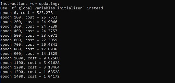
if i%100 == 0:
print("epoch %d, cost = %g" % (i, cost))
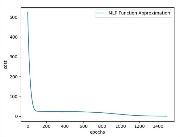
plt.plot(errors,label='MLP Function Approximation') plt.xlabel('epochs')
plt.ylabel('cost')
plt.legend()
plt.show()
输出量
以下是函数层近似的说明-
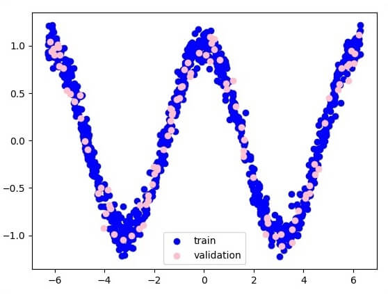
这里,两个数据以W的形式表示。
这两个数据是: train和validate ,它们以不同的颜色描述,如在图例部分中可见。