- R-时间序列分析
- R中的时间序列分析
- R-时间序列分析(1)
- R时间序列分析(1)
- 大数据分析-时间序列分析(1)
- 大数据分析-时间序列分析
- 使用Python的AI –分析时间序列数据
- 使用Python的AI –分析时间序列数据(1)
- 时间序列Python库
- Python时间序列(1)
- 时间序列Python库(1)
- Python时间序列
- 时间序列-编程语言
- 时间序列-编程语言(1)
- Pandas 时间序列
- 算法分析|大O分析(1)
- 算法分析|大O分析
- 算法分析|大O分析
- 时间序列教程(1)
- 时间序列教程
- 时间序列-应用
- 时间序列-应用(1)
- 时间序列-简介
- 时间序列-简介(1)
- 在 R 中合并时间序列(1)
- 在 R 中合并时间序列
- 在 R 编程中使用 ARIMA 模型进行时间序列分析
- 在 R 编程中使用 ARIMA 模型进行时间序列分析(1)
- 讨论时间序列(1)
📅 最后修改于: 2021-01-08 10:09:18 🧑 作者: Mango
R时间序列分析
在规则的时间间隔内测量的任何度量标准都会创建一个时间序列。由于工业上的必要性和相关性,时间序列的分析在商业上很重要,尤其是在预测(需求,供应和销售等)方面。其中每个数据点都与时间戳关联的一系列数据点称为时间序列。
一天中股票在不同时间点的价格是时间序列的最简单示例。一年中不同月份降雨量的另一个例子。 R提供了几个用于创建,处理和绘制时间序列数据的函数。在R对象中,时间序列数据称为时间序列对象。就像矢量或数据帧一样。
创建时间序列
R提供ts()函数来创建时间序列。 ts()函数的语法如下:
Timeseries_object_name<- ts(data, start, end, frequency)
这里,
| S.No | Parameter | Description |
|---|---|---|
| 1. | data | It is a vector or matrix which contains the value used in time series. |
| 2. | start | It is the start time for the first observation |
| 3. | end | It is the end time for the last observation |
| 4. | frequency | It specifies the number of observations per unit time. |
让我们看一个示例,以了解ts()函数如何用于创建时间序列。
例:
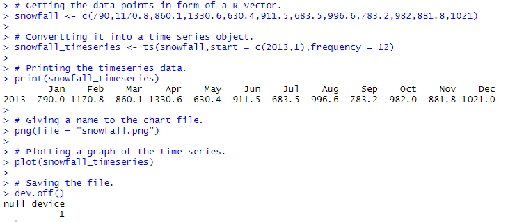
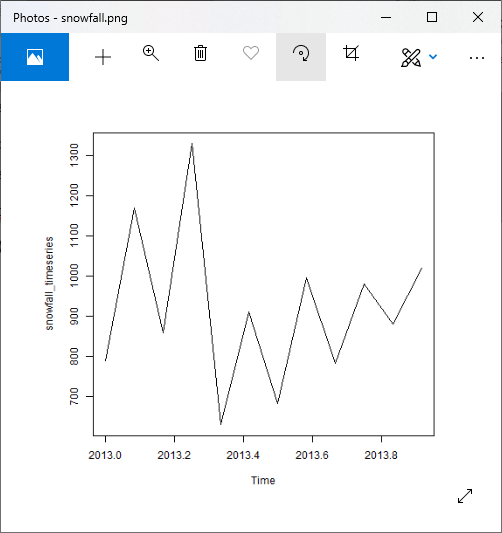
在下面的示例中,我们将考虑从2013年1月开始的某个位置的年度降雪细节。我们将创建一个12个月期间的R时间序列对象,并将其绘制出来。
# Getting the data points in form of a R vector.
snowfall <- c(790,1170.8,860.1,1330.6,630.4,911.5,683.5,996.6,783.2,982,881.8,1021)
# Convertting it into a time series object.
snowfall_timeseries<- ts(snowfall,start = c(2013,1),frequency = 12)
# Printing the timeseries data.
print(snowfall_timeseries)
# Giving a name to the chart file.
png(file = "snowfall.png")
# Plotting a graph of the time series.
plot(snowfall_timeseries)
# Saving the file.
dev.off()
输出:
什么是固定时间序列?
固定时间序列是以下时间序列:
- 时间序列的平均值随时间恒定。这意味着趋势分量被声明为空。
- 差异不应随时间增加。
- 季节性影响应最小。
这意味着它没有季节趋势图样,无论观察到的时间间隔如何,都类似于随机的白噪声。
简而言之,平稳的时间序列是其统计特性(例如均值,方差和自相关等)都随时间恒定的序列。
提取趋势,季节性和误差
我们可以通过将时间序列分为三个部分来分解时间序列,例如季节性,趋势和随机波动。
时间序列分解是将一个时间序列转换成多个时间序列的数学过程。
季节性:
在一段时间内重复的图案
趋势:
矩阵的潜在趋势。
随机:
它是除去季节和趋势序列后原始时间序列的残差。
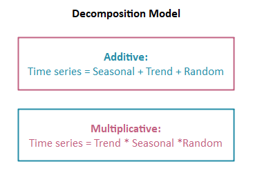
加法和乘法分解
加法和乘法分解是用于分析序列的模型。如果季节性变化似乎是恒定的,则意味着当时间序列的值增加时季节性变化不发生变化,则我们使用加法模型,否则使用乘法模型。
让我们看一个逐步的过程,以了解如何使用加法和乘法模型分解时间序列。对于加性模型,我们使用ausbeer数据集,对于可乘性,我们使用AirPassengers数据集。
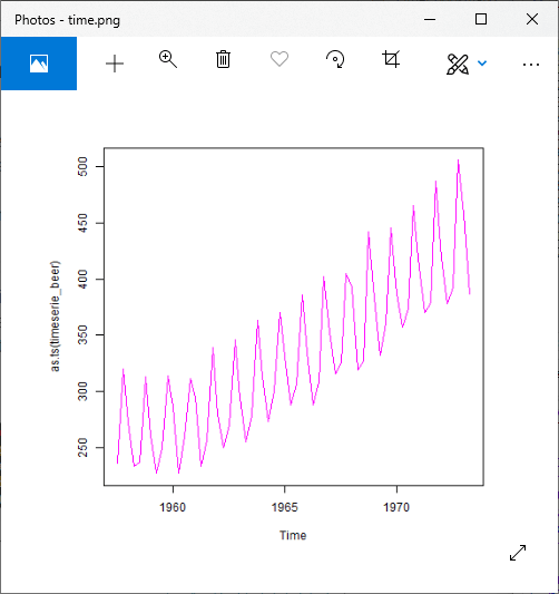
步骤1:加载数据并创建时间序列
对于加性模型
#Importing library fpp
library(fpp)
#Using ausbeer data
data(ausbeer)
#Creating time series for ausbeer dataset
timeserie.beer = tail(head(ausbeer, 17*4+2),17*4-4)
# Giving a name to the chart file.
png(file = "time.png")
plot(as.ts(timeserie_beer), col="magenta")
# Saving the file.
dev.off()
输出:
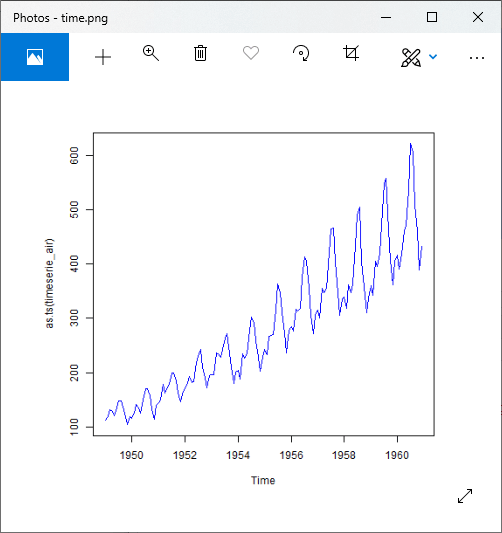
对于乘法模型
#Importing library Ecdat
library(Ecdat)
#Using AirPassengers data
data(AirPassengers)
#Creating time series  for AirPassengers dataset
timeserie_air = AirPassengers
# Giving a name to the file.
png(file = "time.png")
plot(as.ts(timeserie_air))
# Saving the file.
dev.off()
输出:
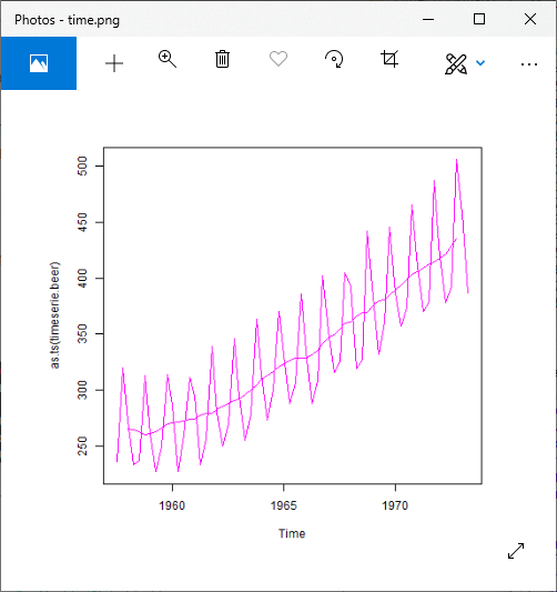
步骤2:检测趋势
对于加性模型
#Detecting trend
trend.beer = ma(timeserie.beer, order = 4, centre = T)
# Giving a name to the file.
png(file = "time.png")
plot(as.ts(timeserie.beer),col="red")
lines(trend.beer,col="red")
plot(as.ts(trend.beer),col="red")
# Saving the file.
dev.off()
输出1:
输出2:

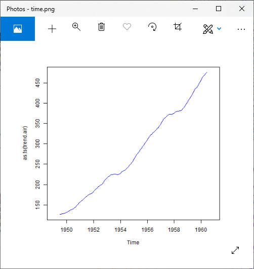
对于乘法模型:
#Detecting trend
trend.air = ma(timeserie.air, order = 12, centre = T)
# Giving a name to the file.
png(file = "time.png")
plot(as.ts(timeserie.air),col="blue")
lines(trend.air,col="blue")
plot(as.ts(trend.air),col="blue")
# Saving the file.
dev.off()
输出1:
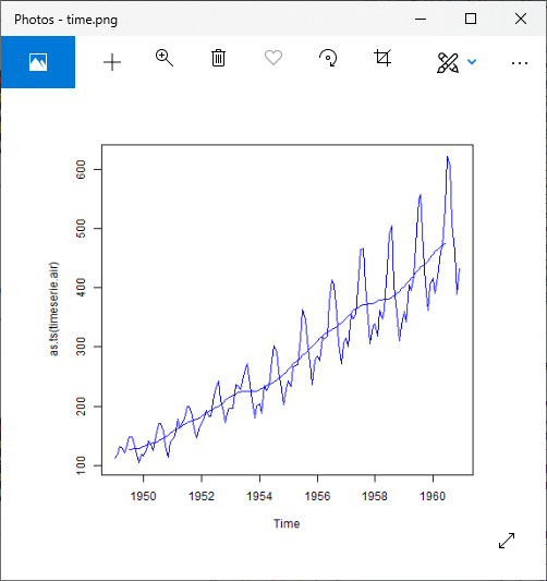
输出2:
步骤3:时间序列趋势
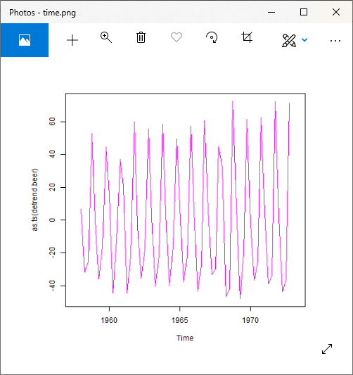
对于加性模型
#Detrend the time series.
detrend.beer=timeserie.beer-trend.beer
# Giving a name to the file.
png(file = "time.png")
plot(as.ts(detrend.beer),col="magenta")
# Saving the file.
dev.off()
输出:
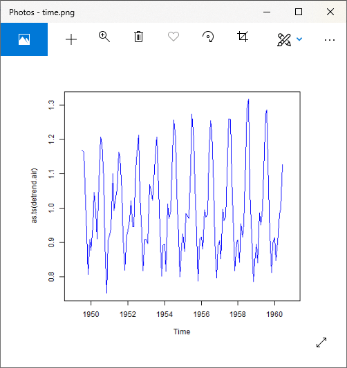
对于乘法模型
#Detrend of time series
detrend.air=timeserie.air / trend.air
# Giving a name to the file.
png(file = "time.png")
plot(as.ts(detrend.air),col="blue")
# Saving the file.
dev.off()
输出:
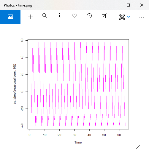
步骤4:平均季节性
对于加性模型
#Average the seasonality
m.beer = t(matrix(data = detrend.beer, nrow = 4))
seasonal.beer = colMeans(m.beer, na.rm = T)
# Giving a name to the file.
png(file = "time.png")
plot(as.ts(rep(seasonal.beer,16)),col="magenta")
# Saving the file.
dev.off()
输出:
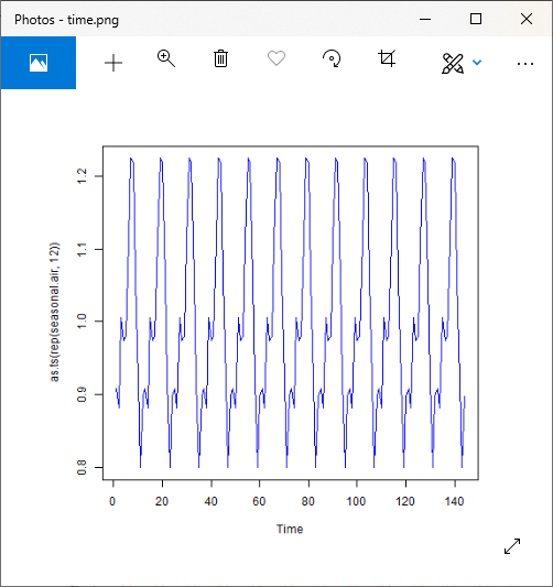
对于乘法模型
#Average the seasonality
m.air = t(matrix(data = detrend.air, nrow = 12))
seasonal.air = colMeans(m.air, na.rm = T)
# Giving a name to the file.
png(file = "time.png")
plot(as.ts(rep(seasonal.air,12)),col="blue")
# Saving the file.
dev.off()
输出:
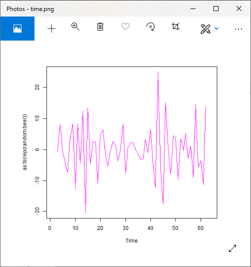
步骤5:检查剩余的随机噪声
对于加性模型
# Examining the Remaining Random Noise
random.beer = timeserie.beer - trend.beer - seasonal.beer
# Giving a name to the file.
png(file = "time.png")
plot(as.ts(rep(random.beer)),col="magenta")
# Saving the file.
dev.off()
输出:
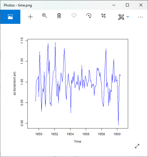
对于乘法模型
# Examining the Remaining Random Noise
random.air = timeserie.air / (trend.air * seasonal.air)
# Giving a name to the file.
png(file = "time.png")
plot(as.ts(random.air),col="blue")
# Saving the file.
dev.off()
输出:
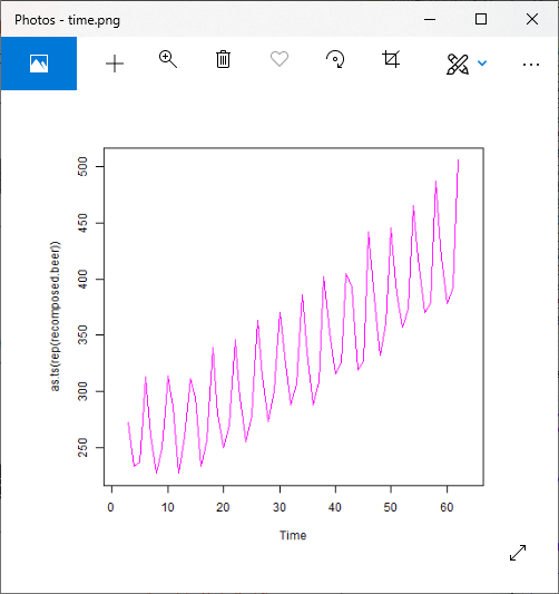
步骤5:重建原始信号
对于加性模型
#Reconstruction of original signal
recomposed.beer=trend.beer+seasonal.beer+random.beer
# Giving a name to the file.
png(file = "time.png")
plot(as.ts(recomposed.beer),col="magenta")
# Saving the file.
dev.off()
输出1:
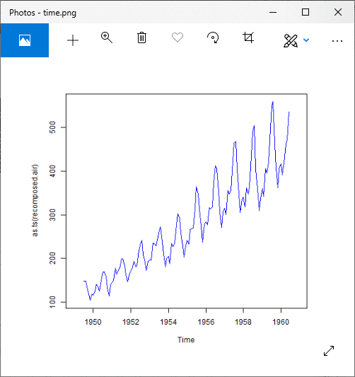
对于乘法模型
#Reconstruction of original signal
recomposed.air = trend.air*seasonal.air*random.air
# Giving a name to the file.
png(file = "time.png")
plot(as.ts(recomposed.air),col="blue")
# Saving the file.
dev.off()
输出:
使用decompose()进行时间序列分解
对于加性模型
#Importing libraries
library(forecast)
library(timeSeries)
library(fpp)
#Using ausbeer data
data(ausbeer)
#Creating time series
timeserie.beer = tail(head(ausbeer, 17*4+2),17*4-4)
#Detect trend
trend.beer = ma(timeserie.beer, order = 4, centre = T)
#Detrend of time series
detrend.beer=timeserie.beer-trend.beer
#Average the seasonality
m.beer = t(matrix(data = detrend.beer, nrow = 4))
seasonal.beer = colMeans(m.beer, na.rm = T)
#Examine the remaining random noise
random.beer = timeserie.beer - trend.beer - seasonal.beer
#Reconstruct the original signal
recomposed.beer = trend.beer+seasonal.beer+random.beer
#Decomposed the time series
ts.beer = ts(timeserie.beer, frequency = 4)
decompose.beer = decompose(ts.beer, "additive")
# Giving a name to the file.
png(file = "time.png")
par(mfrow=c(2,2))
plot(as.ts(decompose.beer$seasonal),col="magenta")
plot(as.ts(decompose.beer$trend),col="magenta")
plot(as.ts(decompose.beer$random),col="magenta")
plot(decompose.beer,col="magenta")
# Saving the file.
dev.off()
输出:
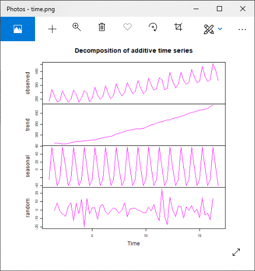
对于乘法模型
#Importing libraries
library(forecast)
library(timeSeries)
library(fpp)
library(Ecdat)
#Using Airpassengers data
data(AirPassengers)
#Creating time series
timeseries.air = AirPassengers
#Detect trend
trend.air = ma(timeseries.air, order = 12, centre = T)
#Detrend of time series
detrend.air=timeseries.air / trend.air
#Average the seasonality
m.air = t(matrix(data = detrend.air, nrow = 12))
seasonal.air = colMeans(m.air, na.rm = T)
#Examine the remaining random noise
random.air = timeseries.air / (trend.air * seasonal.air)
#Reconstruct the original signal
recomposed.air = trend.air*seasonal.air*random.air
#Decomposed the time series
ts.air = ts(timeseries.air, frequency = 12)
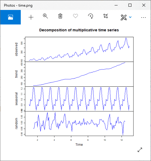
decompose.air = decompose(ts.air, "multiplicative")
# Giving a name to the file.
png(file = "time.png")
par(mfrow=c(2,2))
plot(as.ts(decompose.air$seasonal),col="blue")
plot(as.ts(decompose.air$trend),col="blue")
plot(as.ts(decompose.air$random),col="blue")
plot(decompose.air,col="blue")
# Saving the file.
dev.off()
输出: